Build a Pairs Trading Strategy in Python: A Step-by-Step Guide

Pairs trading is a form of statistical arbitrage that takes advantage of mean reversion or convergence in the prices of two instruments.

The simplest variation of this strategy involves taking long and short positions simultaneously on a pair of cointegrated instruments. But more generally, you can construct a spread from any linear combination of the two instruments with the approach in this tutorial — even going long simultaneously on two instruments.

We’ll make use of the following external libraries:

• databento for market data.
• pandas for data manipulation.
• matplotlib for plotting.
• statsmodels for the Engle-Granger two-step cointegration test.
• scikit-learn to fit the linear regression between the two price series.

import databento as db
import pandas as pd
import matplotlib.pyplot as plt
from statsmodels.tsa.stattools
import coint
from sklearn.linear_model
import LinearRegression

Most existing literature shows the application of this strategy to equities, however the strategy can be applied to any asset class.

We’ll demonstrate the pairs trading strategy on the two most liquid crude oil products traded on CME and ICE, the WTI crude oil futures (CL) and Brent crude oil futures (BRN) contracts respectively.

This also showcases the value of Databento’s supplemental receive timestamps, ts_recv, which are used to construct our OHLCV aggregates. Most academic literature avoids cross-venue arbitrage like this because timestamps from two different exchanges are based on the different reference clocks that cannot be synced easily. ts_recv mitigates this problem by providing a common reference time with sub-microsecond accuracy between geographically-distant venues.

Note: Databento timestamps CME crude and ICE Brent data on the same Aurora I gateway. If you’re using a different data source, you may have to apply a delay offset for the time between Aurora I and 350 E Cermak where their matching engines are situated respectively.

Exchange and clearing fees can be found on CME and ICE’s websites. Tick sizes and notional tick values can be obtained from instrument definitions.

# Instrument-specific configuration
SYMBOL_X = "CLM4"
SYMBOL_Y = "BRN FMN0024!"
TICK_SIZE_X = 0.01
TICK_SIZE_Y = 0.01
TICK_VALUE_X = 10.0
TICK_VALUE_Y = 10.0
FEES_PER_SIDE_X = 0.70      # NYMEX corporate member fees
FEES_PER_SIDE_Y = 0.88

# Global configuration
COMMISSIONS_PER_SIDE = 0.08

# Backtest configuration
START = "2024-04-01"
END = "2024-05-15"

We’ll fetch 1-minute OHLCV aggregates for ease of demonstration, but you may specify schema="mbp-1" to use MBP-1 instead:

def fetch_data():

    client = db.Historical()

    data = client.timeseries.get_range(
        dataset="GLBX.MDP3",
        schema="ohlcv-1m",
        stype_in="raw_symbol",
        symbols=[SYMBOL_X],
        start=START,
        end=END,
    )

    df_x = data.to_df()["close"].to_frame(name="x")

    data = client.timeseries.get_range(
        dataset="IFEU.IMPACT",
        schema="ohlcv-1m",
        stype_in="raw_symbol",
        symbols=[SYMBOL_Y],
        start=START,
        end=END,
    )

    df_y = data.to_df()["close"].to_frame(name="y")

    return df_x.join(df_y, how="outer").ffill()

Since OHLCV aggregates only print when there’s a trade in the interval, you’ll need to use the .ffill() method to synchronize the two time series in cases where one leg doesn't print.

Tip: Although CL and BRN are liquid futures contracts, there’s the possibility that both sides don’t print in a given minute interval. A more complete implementation should resample during every minute of the trading session.

The basis of this strategy is to check that the residuals of a linear regression between the prices of the two instruments exhibits stationarity, also called the Engle-Granger two-step cointegration test. This implies that the two instruments’ price series are cointegrated, and that the spread constructed based on this linear association of the two instruments’ prices is stationary. In turn, this implies that the spread is mean-reverting.

Cointegration is preferred over correlation when constructing a pairs trade, since correlation doesn’t apply to non-stationary time series, and financial instrument prices are typically non-stationary and trending. High correlation between such series can occur even without a meaningful relationship.

For instance, two price series which are trending in the same direction but diverging in the long run may exhibit a spurious, positive correlation.

On the other hand, cointegrated prices series may exhibit positive, negative, or even zero correlation over any period due to short-term fluctuations, but tend to track closely over the long run.

The strategy is simple: First, over the lookback period (last 100 records), we run the cointegration test. If the two series are found to be cointegrated, then the coefficient of linear regression between the two series provides the ratio of the two instruments needed to construct the spread, also called the hedge ratio. We’ll also compute the sample mean and standard deviation over this period.

Then, over the forward window (also 100 records), we compute the spread (residual) and normalize it by taking its z-score.

df = fetch_data()

# Model and monetization parameters
LOOKBACK = 100
ENTRY_THRESHOLD = 1.5
EXIT_THRESHOLD = 0.5
P_THRESHOLD = 0.05

# Initialization
df["cointegrated"] = 0
df["residual"] = 0.0
df["zscore"] = 0.0
df["position_x"] = 0
df["position_y"] = 0
is_cointegrated = False
lr = LinearRegression()

for i in range(LOOKBACK, len(df), LOOKBACK):

    x = df["x"].iloc[i-LOOKBACK:i].values[:,None]
    y = df["y"].iloc[i-LOOKBACK:i].values[:,None]

    if is_cointegrated:
        # Compute and normalize signal on forward window
        x_new = df["x"].iloc[i:i+LOOKBACK].values[:,None]
        y_new = df["y"].iloc[i:i+LOOKBACK].values[:,None]
        spread_back = y - lr.coef_ * x
        spread_forward = y_new - lr.coef_ * x_new
        zscore = (spread_forward - spread_back.mean()) / spread_back.std()
        df.iloc[i:i+LOOKBACK, df.columns.get_loc("cointegrated")] = 1
        df.iloc[i:i+LOOKBACK, df.columns.get_loc("residual")] = spread_forward
        df.iloc[i:i+LOOKBACK, df.columns.get_loc("zscore")] = zscore

    _, p, _ = coint(x,y)
    is_cointegrated = p < P_THRESHOLD
    lr.fit(x,y)

If the normalized residual is negative, it means the instrument associated with y is underpriced, i.e. we’ll buy y and sell x to monetize the prediction that their prices will converge in the future. Conversely, if the normalized residual is positive, we’ll sell y and buy x.

Since the two products have a similar notional value and futures have large minimum order size, we’ll trade a static hedge ratio of 1. If you’re modifying this strategy to trade stocks or ETFs or products that have significant differences in volatility or notional value, you should consider using the dynamic hedge ratio lr.coef_ to scale your position.

Tip: The hedge ratio lr.coef_ may be negative. This regularly occurs, for instance, if one leg of the pair is an inverse ETF.

# Standardized residual is negative => y is underpriced => sell x, buy y
# Standardized residual is positive => y is overpriced => buy x, sell y
df.loc[df.zscore < -ENTRY_THRESHOLD, 'position_y'] = 1
df.loc[df.zscore > ENTRY_THRESHOLD, 'position_y'] = -1
df['position_x'] = -df['position_y']

It’s common to specify a score-based or time-based exit condition. For example, we can exit the position when the spread converges to within +/-0.5 standard deviations. This has the effect of longer holding periods and lower transaction costs.

# Exit positions when z-score crosses +/-0.5
hold_y_long = df["zscore"].apply(lambda z: 1 if z <= -EXIT_THRESHOLD else 0)
hold_y_short = df["zscore"].apply(lambda z: 1 if z >= EXIT_THRESHOLD else 0)

# Carry forward positions until exit condition is met
df["position_y"] = df["position_y"].mask((df["position_y"].shift() == -1) & (hold_y_short == 1), -1)
df["position_y"] = df["position_y"].mask((df["position_y"].shift() == 1) & (hold_y_long == 1), 1)
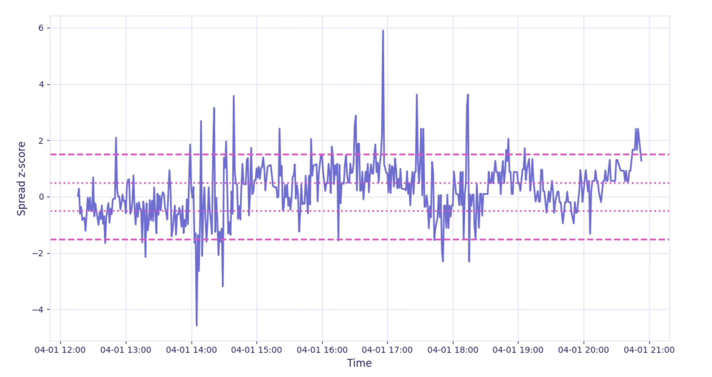
df["position_x"] = -df["position_y"]

Here’s a visualization of the strategy. The outer dashed lines show the entry conditions while the inner dashed lines show the exit conditions:

Exact instantaneous slippage from crossing the spread can be calculated using MBP-1 data and execution timestamps from the backtest. In the interest of time, you can gauge the viability of the strategy by applying a constant spread cost per contract side. This is typically assumed to be half a tick or one tick for liquid futures, but we can also estimate it quickly from a small slice of MBP-1 data:

def estimate_slippage():

    import datetime

    client = db.Historical()

    data = client.timeseries.get_range(
        dataset="GLBX.MDP3",
        schema="mbp-1",
        stype_in="raw_symbol",
        symbols=[SYMBOL_X],
        start=START,
    )

    df = data.to_df()
    avg_spread_x = (df["ask_px_00"] - df["bid_px_00"]).mean()

    data = client.timeseries.get_range(
        dataset="IFEU.IMPACT",
        schema="mbp-1",
        stype_in="raw_symbol",
        symbols=[SYMBOL_Y],
        start=START,
    )

    df = data.to_df()
    avg_spread_y = (df["ask_px_00"] - df["bid_px_00"]).mean()

    return avg_spread_x, avg_spread_y

avg_spread_x, avg_spread_y = estimate_slippage()

We can now compute the gross PnL and transaction costs:

# Compute backtest results
df["pnl_x"] = 0.0
df["pnl_y"] = 0.0
df.iloc[:-1, df.columns.get_loc("pnl_x")] = df['position_x'].iloc[:-1].values * df["x"].diff()[1:].values / TICK_SIZE_X * TICK_VALUE_X
df.iloc[:-1, df.columns.get_loc("pnl_y")] = df['position_y'].iloc[:-1].values * df["y"].diff()[1:].values / TICK_SIZE_Y * TICK_VALUE_Y

df["volume_x"] = df["position_x"].diff().abs()
df["volume_y"] = df["position_y"].diff().abs()
df["tcost"] = df["volume_x"] * FEES_PER_SIDE_X + df["volume_y"] * FEES_PER_SIDE_Y + \
              (df["volume_x"] + df["volume_y"]) * COMMISSIONS_PER_SIDE + \
              (df["volume_x"] * avg_spread_x / TICK_SIZE_X / 2 * TICK_VALUE_X) + \
              (df["volume_y"] * avg_spread_y / TICK_SIZE_Y / 2 * TICK_VALUE_Y).cumsum()
df["gross_pnl"] = (df["pnl_x"] + df["pnl_y"]).cumsum()
df["net_pnl"] = df["gross_pnl"] - df["tcost"]

# Plot and print results
daily_pnl = df["net_pnl"].groupby(df.index.date).sum()
sr = daily_pnl.mean() / daily_pnl.std() * 252**.5
print(f"Sharpe ratio: {sr:.2f}")

plt.plot(df["gross_pnl"], label="Gross PnL")
plt.plot(df["net_pnl"], label="Net PnL")
plt.plot(df["tcost"], label="t-cost")
plt.xlabel("Date")
plt.ylabel("PnL (USD)")
plt.legend()
plt.show()

Sharpe ratio: 8.57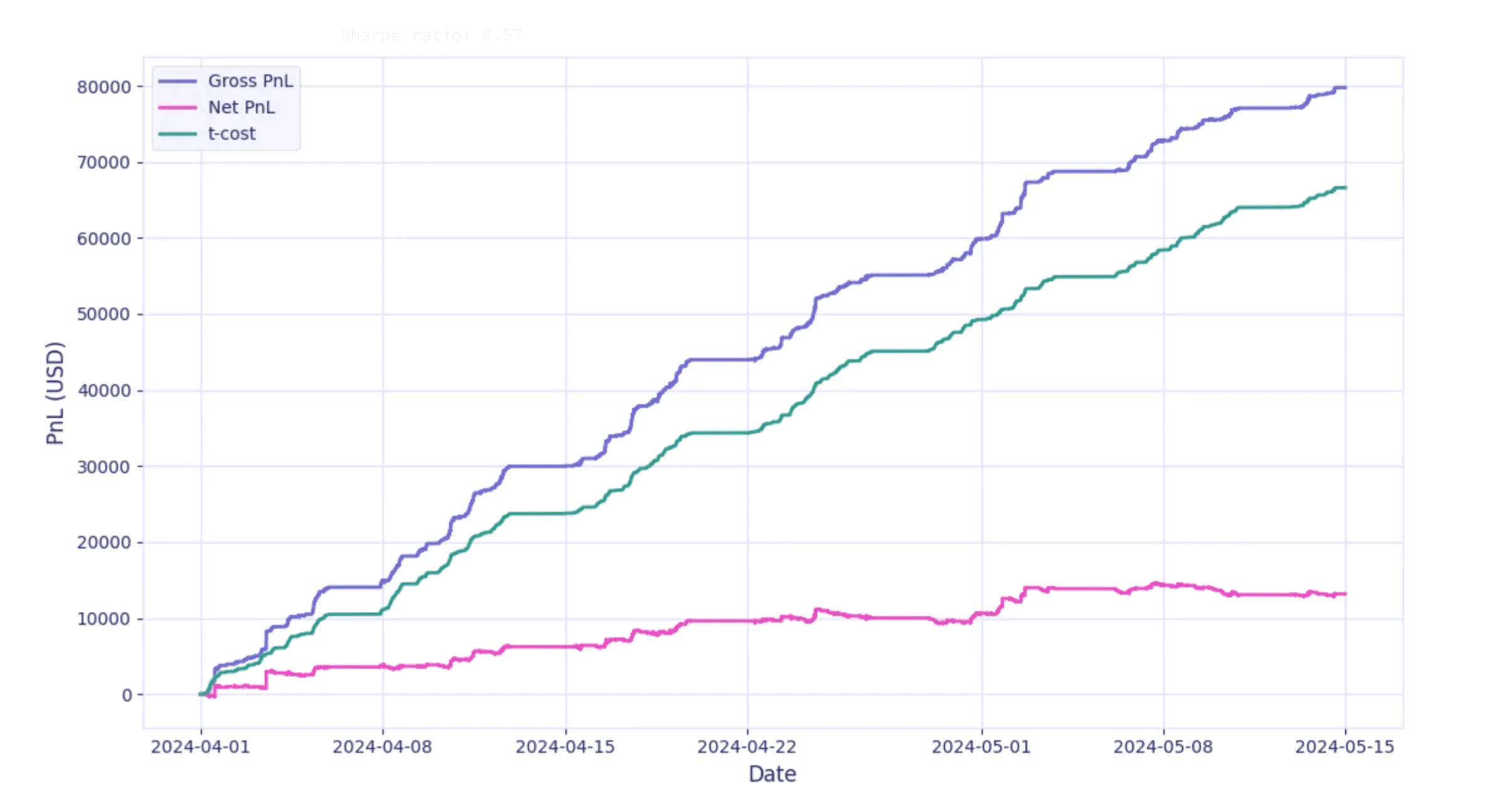

The full code example can be found on our GitHub here.

This tutorial is kept intentionally short using a simple vectorized implementation. Ideally, you should use MBP-1 data with an event-driven backtest loop that incorporates the delays between your system and the exchange gateways. This can be done using the market replay method.

This strategy is very sensitive to slippage and the exact expiration month that’s traded; non-lead month contracts will have wider spreads which can make the strategy infeasible.

We assumed exchange fees and commissions that are realistic for a medium-sized trading firm or a team within a larger firm that’s already a CME member firm. In practice, achieving similar rates requires a NYMEX 106.J corporate membership and thousands of contract sides executed per day.

Scaling up to larger trade sizes will significantly expand the strategy’s state machine, since you’ll have to handle partial executions and different sizes on each leg of the spread to achieve optimal hedge ratio. MBP-1 data can also inform trade sizing.

We introduced a few free model and monetization parameters, namely LOOKBACK, ENTRY_THRESHOLD, EXIT_THRESHOLD. These can be optimized using any hyperparameter tuning method (e.g. grid search) and cross-validated.

There are also a few common variations of this strategy to consider:

• Basket trading by constructing combinations of more than two instruments, using another procedure such as the Johansen test.
• Calibrating an Ornstein-Uhlenbeck process, which gives a parametric model for time-based exit.
• Using total least squares instead of ordinary least squares to determine the hedge ratio.
• Scanning a wide universe systematically for cointegrated pairs, to discover unintuitive relationships. However, this runs the risk of poor generalization if too many pairs are tested. Dimensionality reduction methods like PCA can improve the search and generalization error.

Alexander, C. (2008). Market Risk Analysis: Practical Financial Econometrics (Vol. 2). Wiley.

Tsay, R. S. (2010). Analysis of Financial Time Series (3rd edition). Wiley.

Engle, R. F., & Granger, C. W. J. (1987). Co-integration and error correction: Representation, estimation, and testing. Econometrica, 55(2), 251–276.