Computing the option Greeks using Pathway and Databento

May 20, 2025

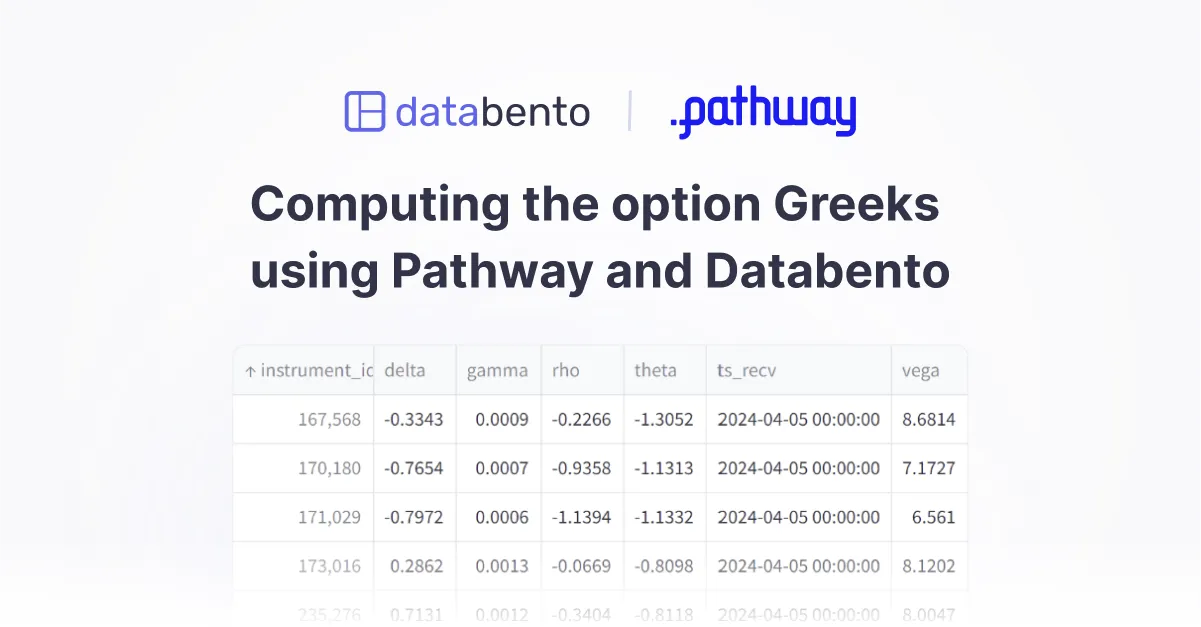
This tutorial from the team at Pathway demonstrates how to compute option Greeks using Databento’s real-time and historical CME data. It applies the Black-76 model—a variation of Black-Scholes designed for pricing European-style options on futures—to calculate five key option Greeks: Delta, Gamma, Theta, Vega, and Rho.

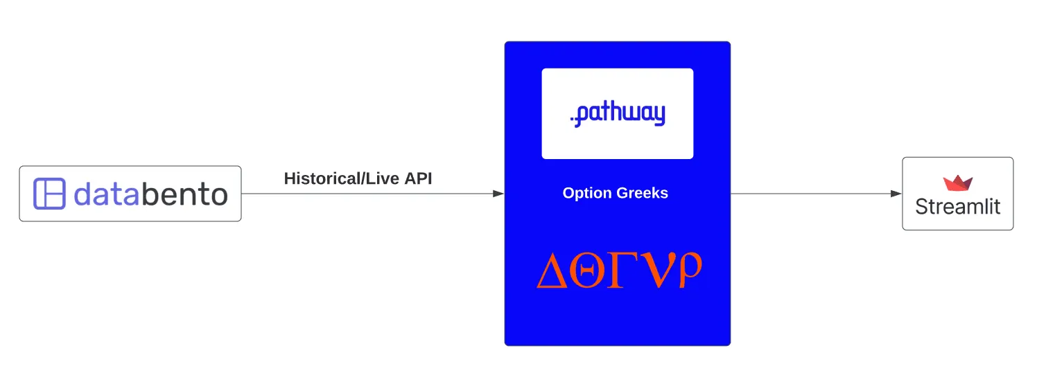
It builds on our documentation example for estimating implied volatility with historical data and shows how the same pricing model can be implemented in a real-time ETL pipeline using Pathway, a Python framework for building streaming data applications. In this setup, Pathway ingests market data from Databento, processes it through the Black-76 pricing model, and continuously streams updated values for each Greek. Pathway’s engine supports both historical and live data, making it well-suited for backtesting and real-time trading workflows.

You can find the complete code on GitHub, or skip ahead to the tutorial here.

Before diving into Pathway’s step-by-step guide, there are a few important nuances to consider when calculating option Greeks.

Greeks rely on inputs that update at different intervals and vary in granularity. Some values can be reused across contracts with the same expiration, while others must be calculated for each strike or exercise style.

They're also highly sensitive to model assumptions and parameters, many of which reflect practical observations of market microstructure that aren’t captured in academic texts or theoretical models. Because data providers often overlook these effects—particularly those related to instrument-specific behaviors like early exercise and dividends—most trading firms prefer to calculate their own Greeks for greater control over the assumptions that drive their pricing and risk models.

Although the European-style options on futures used in this example are among the simplest to model, they still involve baseline assumptions that can vary depending on your strategy:

This pipeline assumes 252 trading days per year, but using an exchange-specific calendar can provide a more precise measure of time to expiration.
It also uses a fixed 4.3% risk-free interest rate. Alternatively, you can derive a short-term spot rate from real-time SOFR futures to better reflect market expectations.

More complex instruments introduce additional modeling challenges:

Equity options require switching to models like Black-Scholes or SVI and incorporating dividend estimates from corporate actions data.
American-style options, which can be exercised early, fall outside the scope of closed-form models and typically require numerical methods to estimate the optimal time to exercise.

These considerations highlight why we haven't adopted a one-size-fits-all approach to providing Greeks. Accurate calculation depends on a mix of modeling choices, market assumptions, and instrument-specific variables that differ by asset class and strategy. Pipelines like Pathway's offer the flexibility needed to adjust the logic to your specific requirements.

Options are financial derivatives that give the holder the right, but not the obligation, to buy or sell an underlying asset at a specified price within a certain period. On the other hand, futures are contracts that obligate the parties involved to buy or sell an asset at a predetermined price on a specified future date. Options are commonly used in various financial strategies, including hedging and speculation.

In this tutorial, you are going to manipulate options on futures.

There are two kind of options: (1) call options and (2) put options. A call option gives the holder the right, but not the obligation, to buy the underlying asset at a specified price (the strike price) before or at the option's expiration date. On the other hand, a put option gives the holder the right, but not the obligation, to sell the underlying asset at the strike price before or at the expiration date.

In options trading, option Greeks are metrics used to assess the sensitivity of option prices and provide detailed, quantifiable measures of various risk factors. Using option Greeks, traders and risk managers make more informed, strategic decisions, enhancing their ability to manage risk and optimize returns.

Each option Greek measures the sensisibility of option prices to different factors:

Delta $(Δ)$ measures the change in an option's price relative to the change in the underlying asset's price. For a call option, Delta is positive, ranging from 0 to 1. This is because as the underlying asset's price increases, the call option becomes more valuable. For a put option, Delta is negative, ranging from -1 to 0. This is because as the underlying asset's price decreases, the put option becomes more valuable.
Gamma $(Γ)$ indicates the rate of change of Delta with respect to changes in the price of the underlying asset for both calls and puts. A high Gamma indicates that Delta can change rapidly. Monitoring Gamma helps in understanding how stable an option's Delta is.
Theta $(Θ)$ represents the time decay of an option. For call options, Theta is usually negative, indicating the option loses value as time passes, given all else remains constant. For put options, Theta is also negative, but the rate at which the value decays can differ because the time decay effect can be more pronounced in different market conditions and volatilities.
Vega $(V)$ measures sensitivity to volatility for both calls and puts. Higher volatility increases the value of both calls and puts, but the degree can vary depending on whether it's a call or a put and their respective positions relative to the strike price.
Rho $(ρ)$ indicates sensitivity to interest rate changes. For call options, Rho is positive, meaning the value of a call option increases as interest rates rise. For put options, Rho is negative, meaning the value of a put option decreases as interest rates rise.

These metrics help traders and risk managers understand and hedge the risks associated with options positions. You can learn more about option Greeks here.

First, let's introduce some notations. Let's define $d_{1}, d_{2}$ to help us define the Greeks. Here,

$F$ is the futures price, the agreed-upon price in a futures contract between 2 parties, of an asset, at a specified time in the future
$K$ is the strike price, the price at which one can sell/buy that option,
$T$ is the time to expiration in years,
$r$ is the risk-free interest rate, the theoretical rate of return of an investment with zero risk,
$σ$ is the volatility, the variation of prices over some time interval, also known as the standard deviation of logarithmic returns,
$N (x)$ is the standard normal cumulative distribution function,
$N' (x)$ is the standard normal probability density function.

d_{1} = \frac{ln ( \frac{F}{K} ) + ( 0.5 \cdot σ ^{2} ) T}{σ T}, d_{2} = d_{1} - σ T

The option Greeks are defined using $d_{1}$ and $d_{2}$ . Formula changes depending on whether the option is a call or a put.

Call option: $Δ = e^{- r T} N (d_{1})$
Put option: $Δ = - e^{- r T} N (- d_{1})$

For both call and put options: $Γ = e^{- r T} \frac{N ^{'} ( d _{1} )}{S σ T}$

For call option: $Θ = \frac{\frac{- F σ N ^{'} ( d _{1} )}{2 T} - r \cdot K \cdot e ^{- r T} N ( d _{2} ) + r \cdot F \cdot e ^{- r T} N ( d _{1} )}{252}$
For put option: $Θ = \frac{\frac{- F σ N ^{'} ( d _{1} )}{2 T} + r \cdot K \cdot e ^{- r T} N ( - d _{2} ) - r \cdot F \cdot e ^{- r T} N ( - d _{1} )}{252}$

For both call and put options: $V = e^{- r T} \frac{F \cdot N ^{'} ( d _{1} ) T}{100}$

For call option: $ρ = - T e^{- r T} \frac{F \cdot N ( d _{1} ) - K \cdot N ( d _{2} )}{100}$
For put option: $ρ = - T e^{- r T} \frac{K \cdot N ( - d _{2} ) - F \cdot N ( - d _{1} )}{100}$

First, you need financial data. Stock market data is usually public and can be accessed using APIs. Databento provides simple and fast Python APIs to access market data. You can signup and get free credits. You will obtain an API key with your account: save it, you will need it to access the data.

To continue, make sure to install all the needed packages.

!pip install pathway databento pandas scipy numpy python-dotenv

Let's start by importing Pathway and Databento:

import databento as db
import pathway as pw

You need to use the API key to access Databento's data. You can create an .env file and set an environment variable or paste the API key directly into the code.

To use the .env file, you first need to create the file, and then copy the key directly in the file:

API_KEY = "********"

Then, you need to use the os package to load the variable:

import os
from dotenv import load_dotenv

load_dotenv()
API_KEY = os.environ.get("API_KEY")
client = db.Historical(API_KEY)

Let's start with static data and switch to streaming once everything is ready. Both Databento and Pathway make switching to streaming very easy.

Let's focus on E-mini S&P 500 futures contracts whose associated symbol is ES. The data is from the Globex exchange platform of the CME Group.

Options are represented by a specific formatting: root symbol + month + year then type + strike price. Let's take ESM4 C2950 as an example:

Its root symbol is ES, it is a E-mini S&P 500 future contract.
M4 refers to the expiration month and year of the contract: it expires in June 2024.
C means that it is a call option. P is used for puts.
2950 is the strike price of the option. It is the prices at which the holder can buy the ESM4 future contract.

ESM4 is called the underlying asset of the of the option, it is the E-mini S&P 500 futures contract that expires in June 2024.

The data is separated into two datasets: the definitions and the orders.

Definitions provides reference information about each instrument. For options, you are going to use those:

The symbol of option.
The identifier of the option.
The underlying future.
The type of option.
The expiration time of the option.
The strike price of the option.
The time of reception of the data.

This data is static by nature and do not change over time.

In addition to the definitions, you also need the state of the market. You will use the order book. For options, you will need:

The symbol of the option.
The bid price.
The ask price.

You won't need the times of the order as only the orders from the requested time slot will be received. The book order data is dynamic by nature as new orders arrive over time. However, this article will focus on querying historical data: past orders from a given time period. This data is static as it is data from a given time period: all the orders of this time period are known and included in the data.

The CME Globex data can be found in the GLBX.MDP3 dataset and the definition schema. This provides us with useful information about our options, such as the option type or expiration time of the future.

db_dataset = "GLBX.MDP3" # CME Globex MDP 3.0
db_def_schema = "definition" # this provides us the reference information of each instrument
db_def_symbols = ["ES.OPT"] # all options whose root symbol is ES

For historical data, the start time and duration are also needed:

import pandas as pd

start_time = pd.Timestamp("2024-04-04T17:00:00", tz="Us/Central")
data_duration = pd.Timedelta(days=1)

Let's define a custom Pathway connector, to read the data directly from Databento's API. First, you need to declare the schema of the data:

class DefinitionInputSchema(pw.Schema):
    ts_recv: int          # time in ns when the data was received
    raw_symbol: str       # symbol of option
    expiration: int       # expiration time of the option
    instrument_class: str # type of option
    strike_price: float   # see below for what it means
    underlying: str       # symbol of the first underlying instrument
    instrument_id: int    # An identifier of the option

Now, you need to define a ConnectorSubject that will define how the data is read and ingested by Pathway. The market data is accessed in the ConnectorSubject using Databento's time series:

class DefinitionSubject(pw.io.python.ConnectorSubject):
    def run(self):
        # First, get Databento's data:
        data = client.timeseries.get_range(
            dataset=db_dataset,
            schema=db_def_schema,
            symbols=db_def_symbols,
            stype_in=db.SType.PARENT,
            start=start_time,
            end=start_time + data_duration,
        )
        # Now, ingest the data into Pathway:
        for row in data:
            # Get the attributes you are interested in
            ts_recv = getattr(row, "ts_recv")
            raw_symbol = getattr(row, "raw_symbol")
            expiration = getattr(row, "expiration")
            instrument_class = getattr(row, "instrument_class")
            strike_price = getattr(row, "strike_price") / 1e9
            underlying = getattr(row, "underlying")
            instrument_id = getattr(row, "instrument_id")

            # Transmit the data
            self.next(
                ts_recv=ts_recv,
                raw_symbol=raw_symbol,
                expiration=expiration,
                instrument_class=instrument_class,
                strike_price=strike_price,
                underlying=underlying,
                instrument_id=instrument_id,
            )

You can read more about how to access Databento data in our Documentation.

Now you can create the table using the Python connector:

table_es = pw.io.python.read(DefinitionSubject(), schema=DefinitionInputSchema)

            | ts_recv             | raw_symbol        | expiration          | instrument_class | strike_price      | underlying | instrument_id
^NQ4SN5H... | 1712268100558405731 | UD:1V: SG 2766914 | 1712354340000000000 | T                | 9223372036.854776 |            | 2766914
^TKNWB16... | 1712268121809444020 | UD:1V: GN 2766927 | 1712354340000000000 | T                | 9223372036.854776 |            | 2766927
^QPDB24M... | 1712269634334772214 | UD:1V: 12 2767163 | 1712354340000000000 | T                | 9223372036.854776 |            | 2767163
^5HSNPF6... | 1712269897918754155 | UD:1V: VT 2767198 | 1712354340000000000 | T                | 9223372036.854776 |            | 2767198
^3EH930P... | 1712270087811250835 | UD:1V: GT 2767215 | 1712354340000000000 | T                | 9223372036.854776 |            | 2767215

Currently, your table contain all the options. You need to keep only the one you are interested in. Among all the futures corresponding to the associated future ES, let's focus on ESM4. In practice you may be interested in the front-month symbol, the one that has the closest expiration date.

front_month_symbol = 'ESM4'

Let's filter the data to only keep the options associated with ESM4 futures. To only compute the Greeks for the correct options, let's filter out all those whose underlying instrument is different from ESM4:

table_esm4 = table_es.filter(pw.this.underlying==front_month_symbol)

            | ts_recv             | raw_symbol | expiration          | instrument_class | strike_price | underlying | instrument_id
^9JKNAD4... | 1712275200000000000 | ESM4 C0055 | 1718976600000000000 | C                | 55.0         | ESM4       | 42409251
^4BKX67J... | 1712275200000000000 | ESM4 C0100 | 1718976600000000000 | C                | 100.0        | ESM4       | 42406524
^SB2J9YB... | 1712275200000000000 | ESM4 C0200 | 1718976600000000000 | C                | 200.0        | ESM4       | 42439016
^CVV6ENZ... | 1712275200000000000 | ESM4 C0300 | 1718976600000000000 | C                | 300.0        | ESM4       | 42439018
^HRK3X6X... | 1712275200000000000 | ESM4 C0700 | 1718976600000000000 | C                | 700.0        | ESM4       | 129750

As a safeguard, let's also filter on the instrument_class to make sure the value is either C (CALL) or P (PUT):

table_esm4 = table_esm4.filter((pw.this.instrument_class == 'C') | (pw.this.instrument_class == 'P'))

            | ts_recv             | raw_symbol | expiration          | instrument_class | strike_price | underlying | instrument_id
^9JKNAD4... | 1712275200000000000 | ESM4 C0055 | 1718976600000000000 | C                | 55.0         | ESM4       | 42409251
^4BKX67J... | 1712275200000000000 | ESM4 C0100 | 1718976600000000000 | C                | 100.0        | ESM4       | 42406524
^SB2J9YB... | 1712275200000000000 | ESM4 C0200 | 1718976600000000000 | C                | 200.0        | ESM4       | 42439016
^CVV6ENZ... | 1712275200000000000 | ESM4 C0300 | 1718976600000000000 | C                | 300.0        | ESM4       | 42439018
^HRK3X6X... | 1712275200000000000 | ESM4 C0700 | 1718976600000000000 | C                | 700.0        | ESM4       | 129750

Now that you have the options, you need to find the associated orders. The prices, used to compute the volatility, are obtained by averaging all the bids and ask prices. Hence, mid-price is the correct term.

This data will be obtained from the mbp-1 schema (Market by price), which provides every event that updates the top price.

To limit data usage, you can query only the symbols present in your data:

table_symbols = table_esm4.reduce(symbol_tuple = pw.reducers.tuple(pw.this.raw_symbol))
symbol_list = [front_month_symbol] + list(pw.debug.table_to_pandas(table_symbols)['symbol_tuple'][0])

As an example, let's only query over a 2 minutes time interval, to limit the number of data to extract and process. Similarly to the definition schema, you will use a custom connector to read the data from Databento:

db_price_schema = "mbp-1"

class MBP1InputSchema(pw.Schema):
    raw_symbol: str # the symbol of the option
    bid_px: float   # the bid price
    ask_px: float   # the ask price

# Only 2 minutes
query_data_duration = pd.Timedelta(minutes=2)

class MBP1Subject(pw.io.python.ConnectorSubject):
    def run(self):
        data = client.timeseries.get_range(
            dataset=db_dataset,
            schema=db_price_schema,
            start=start_time,
            end=start_time + query_data_duration,
            symbols=symbol_list
        )
        # Databento's instrument map, which will help us get the symbols from the row data
        instrument_map = db.common.symbology.InstrumentMap()
        instrument_map.insert_metadata(data.metadata)
        for row in data:
            symbol = instrument_map.resolve(row.instrument_id, row.pretty_ts_recv.date())
            levels = getattr(row, "levels")
            # INT64_MAX is the mark for unknown bid/ask prices
            if levels[0].bid_px > (1 << 63) - 10 or levels[0].ask_px > (1 << 63) - 10:
                continue
            # Prices unit is actually 1e-9
            bid_px = levels[0].bid_px / 1e9
            ask_px = levels[0].ask_px / 1e9
            self.next(
                raw_symbol=symbol,
                bid_px=bid_px,
                ask_px=ask_px,
            )

table_mbp1 = pw.io.python.read(MBP1Subject(), schema=MBP1InputSchema)

            | raw_symbol | bid_px  | ask_px
^Z4T8WTR... | ESM4       | 5199.75 | 5200.0
^R8ZACFQ... | ESM4       | 5199.75 | 5200.0
^VM93KP5... | ESM4       | 5199.75 | 5200.0
^PX3Z53V... | ESM4       | 5199.75 | 5200.0
^3A5E19T... | ESM4       | 5199.75 | 5200.0

To compute the average prices for all bids, you can use a simple groupby/reduce:

table_mbp1 = table_mbp1.groupby(pw.this.raw_symbol).reduce(
    raw_symbol=pw.this.raw_symbol,
    option_midprice=(pw.reducers.avg(pw.this.bid_px) + pw.reducers.avg(pw.this.ask_px)) / 2,
)

            | raw_symbol | option_midprice
^QT4BK1X... | ESM4       | 5203.894756928135
^6ZHHRC0... | ESM4 C3950 | 1255.875
^W641MZJ... | ESM4 C4000 | 1206.25
^WGH73K1... | ESM4 C4050 | 1156.75
^HWYWY52... | ESM4 C4100 | 1107.25

Now, you want to add the data from the table_esm4 to this table_mbp1. To do so, you need to join the two table on the raw_symbol values:

table_prices = table_esm4.join(
    table_mbp1,
    pw.left.raw_symbol == pw.right.raw_symbol
).select(
    *pw.left,  # Adding all the columns from table_esm4
    option_midprice=pw.right.option_midprice,
)

            | ts_recv             | raw_symbol | expiration          | instrument_class | strike_price | underlying | instrument_id | option_midprice
^6ZHYYVZ... | 1712275200000000000 | ESM4 C3950 | 1718976600000000000 | C                | 3950.0       | ESM4       | 4162742       | 1255.875
^W64CERT... | 1712275200000000000 | ESM4 C4000 | 1718976600000000000 | C                | 4000.0       | ESM4       | 574893        | 1206.25
^WGHCM9D... | 1712275200000000000 | ESM4 C4050 | 1718976600000000000 | C                | 4050.0       | ESM4       | 4162333       | 1156.75
^HWYHF5C... | 1712275200000000000 | ESM4 C4100 | 1718976600000000000 | C                | 4100.0       | ESM4       | 655090        | 1107.25
^GGRY3PT... | 1712275200000000000 | ESM4 C4150 | 1718976600000000000 | C                | 4150.0       | ESM4       | 4162743       | 1058.0

Now that the data is ready, you can compute the option Greeks. To do so, you need several values, as you have seen in the Generic Formulas section. Recall that you need:

$F,$ the futures price
$K,$ the strike price
$T,$ the time to expiration
$r,$ the risk-free interest rate
$σ,$ the volatility.

This is a bit more complicated, as it is usually determined by the market and is taken from government securities considered free of default risk. This can be considered more of an input parameter given by the user.

Let's use $0.043$ as the value for this interest rate, based on government available data.

interest_rate = 0.043

In the Black/Black 76 Model, the option Greeks are the options of the front-month contract, this value will be fixed per each front-month contract. In this case, it will be the stock price/last price of the ESM4 option. You can access rows by value using ix_ref:

table_prices = table_prices.with_columns(
    future_price=table_mbp1.ix_ref(front_month_symbol).option_midprice
)

            | ts_recv             | raw_symbol | expiration          | instrument_class | strike_price | underlying | instrument_id | option_midprice | future_price
^6ZHYYVZ... | 1712275200000000000 | ESM4 C3950 | 1718976600000000000 | C                | 3950.0       | ESM4       | 4162742       | 1255.875        | 5203.894756928135
^W64CERT... | 1712275200000000000 | ESM4 C4000 | 1718976600000000000 | C                | 4000.0       | ESM4       | 574893        | 1206.25         | 5203.894756928135
^WGHCM9D... | 1712275200000000000 | ESM4 C4050 | 1718976600000000000 | C                | 4050.0       | ESM4       | 4162333       | 1156.75         | 5203.894756928135
^HWYHF5C... | 1712275200000000000 | ESM4 C4100 | 1718976600000000000 | C                | 4100.0       | ESM4       | 655090        | 1107.25         | 5203.894756928135
^GGRY3PT... | 1712275200000000000 | ESM4 C4150 | 1718976600000000000 | C                | 4150.0       | ESM4       | 4162743       | 1058.0          | 5203.894756928135

Using the expiration column, you can compute the time to expiration $T$ which is used in our formulas. Because of how the formulas are defined, it is expressed in years.

Be careful, the unit of expiration is nanoseconds.

# Compute the time to expiration, has to be in years
@pw.udf
def compute_time_to_expiration(expiration_time: int) -> float:
    return (expiration_time - int(start_time.timestamp() * 1e9)) / (1e9 * 86400 * 365)


table_texp = table_prices.with_columns(
    time_to_expiration=compute_time_to_expiration(pw.this.expiration)
)

            | ts_recv             | raw_symbol | expiration          | instrument_class | strike_price | underlying | instrument_id | option_midprice | future_price      | time_to_expiration
^6ZHYYVZ... | 1712275200000000000 | ESM4 C3950 | 1718976600000000000 | C                | 3950.0       | ESM4       | 4162742       | 1255.875        | 5203.894756928135 | 0.2127283105022831
^W64CERT... | 1712275200000000000 | ESM4 C4000 | 1718976600000000000 | C                | 4000.0       | ESM4       | 574893        | 1206.25         | 5203.894756928135 | 0.2127283105022831
^WGHCM9D... | 1712275200000000000 | ESM4 C4050 | 1718976600000000000 | C                | 4050.0       | ESM4       | 4162333       | 1156.75         | 5203.894756928135 | 0.2127283105022831
^HWYHF5C... | 1712275200000000000 | ESM4 C4100 | 1718976600000000000 | C                | 4100.0       | ESM4       | 655090        | 1107.25         | 5203.894756928135 | 0.2127283105022831
^GGRY3PT... | 1712275200000000000 | ESM4 C4150 | 1718976600000000000 | C                | 4150.0       | ESM4       | 4162743       | 1058.0          | 5203.894756928135 | 0.2127283105022831

The volatility represents the market's expectation of the future volatility of the underlying asset over the life of the option. Unlike historical volatility, which measures past price fluctuations, implied volatility is derived from the market price of the option itself.

Using the Black Model, you can infer volatility using known data. The option price will be estimated as being the average of the prices associated to that option symbol. You need to compute σ (the volatility) so that the price calculated in the Black Model is the same as the estimated option price. It comes down to finding the root of a polynomial, which will be done using scipy.

What follows next is just the previous formulas being translated into Python.

First, you need to define the function to compute the option price in the Black Model, having computed the volatility, σ.

import math

def compute_price(
    F: float,
    K: float,
    T: float,
    sigma: float,
    r: float=interest_rate,
    is_call: bool=True
) -> float:
    d1 = (math.log(F / K) + (sigma**2 / 2) * T) / (sigma * math.sqrt(T))
    d2 = d1 - sigma * math.sqrt(T)
    sign = 2 * int(is_call) - 1

    return math.exp(-r * T) * sign * (norm.cdf(sign * d1) * F - norm.cdf(sign * d2) * K)

Now, solve the equation by finding the roots of

BlackPrice (σ) - MeanPrice = 0

using scipy's root finding function. To mark the non-convergence/non-existence of a root, return $N o n e$ .

import scipy
from scipy.stats import norm

@pw.udf
def compute_volatility(
    F: float,
    K: float,
    T: float,
    _is_call: bool,
    option_midprice: float
) -> float | None:
    result = scipy.optimize.root_scalar(
        lambda sigma: option_midprice - compute_price(
            F=F,
            K=K,
            T=T,
            sigma=sigma,
            is_call=_is_call
        ),
        x0=0.0001,x1=0.8
    )

    return result.root if result.converged else None

Now, let's compute the $d_{1}, d_{2}$ defined as before. Let's define those functions as Pathway user-defined function using the pw.udf decorator. Another alternative would be to declare the functions as simple Python functions and apply them to the columns using pw.apply.

@pw.udf
def compute_d1(
    F: float,
    K: float,
    T: float,
    sigma: float,
    r: float = interest_rate,
) -> float:
    return (math.log(F / K) + (sigma**2 / 2) * T) / (sigma * math.sqrt(T))

@pw.udf
def compute_d2(
    F: float,
    K: float,
    T: float,
    sigma: float,
    r: float = interest_rate
) -> float:
    return (math.log(F / K) + (sigma**2 / 2) * T) / (sigma * math.sqrt(T)) - sigma * math.sqrt(T)

You can now define the functions to compute the option Greeks using $F, K, T, σ, d_{1}, d_{2},$ and $ρ :$

@pw.udf
def compute_delta(F: float, K: float, T: float, sigma: float, d1: float, d2: float, is_call: bool, r: float = interest_rate) -> float:
    return math.exp(-r * T) * norm.cdf(d1) if is_call \
           else -math.exp(-r * T) * norm.cdf(-d1)

@pw.udf
def compute_gamma(F: float, K: float, T: float, sigma: float, d1: float, d2: float, is_call: bool, r: float = interest_rate) -> float:
    return math.exp(-r * T) * norm.pdf(d1) / (F * sigma * math.sqrt(T))

@pw.udf
def compute_theta(F: float, K: float, T: float, sigma: float, d1: float, d2: float, is_call: bool, r: float = interest_rate) -> float:
    return (-F * sigma * norm.pdf(d1) / (2 * math.sqrt(T)) - r * K * math.exp(-r * T) * norm.cdf(d2) + r * F * math.exp(-r * T) * norm.cdf(d1)) / 252 if is_call \
           else (-F * sigma * norm.pdf(d1) / (2 * math.sqrt(T)) + r * K * math.exp(-r * T) * norm.cdf(-d2) - r * F * math.exp(-r * T) * norm.cdf(-d1)) / 252# per day

@pw.udf
def compute_vega(F: float, K: float, T: float, sigma: float, d1: float, d2: float, is_call: bool, r: float = interest_rate) -> float:
    return F * norm.pdf(d1) * math.sqrt(T) * math.exp(-r * T) / 100

@pw.udf
def compute_rho(F: float, K: float, T: float, sigma: float, d1: float, d2: float, is_call: bool, r: float = interest_rate) -> float:
    return -T * math.exp(-r * T) * (F * norm.cdf(d1) - K * norm.cdf(d2)) / 100 if is_call \
           else -T * math.exp(-r * T) * (K * norm.cdf(-d2) - F * norm.cdf(-d1)) / 100

All you need to do is to use the UDFs you have just defined.

First, let's add a column to determine if the option is a call or a put:

table_texp = table_texp.with_columns(is_call=pw.this.instrument_class == 'C')

Now, you can start computing the options Greeks. First, let's start with the implied volatility, pre-filtering.

table_volatility_unfiltered = table_texp.with_columns(
    volatility=compute_volatility(
        pw.this.future_price,
        pw.this.strike_price,
        pw.this.time_to_expiration,
        pw.this.is_call,
        pw.this.option_midprice
    )
)

Filter out entries were volatility couldn't be computed.

table_sigma = table_volatility_unfiltered.filter(pw.this.volatility.is_not_none())

            | ts_recv             | raw_symbol | expiration          | instrument_class | strike_price | underlying | instrument_id | option_midprice | future_price      | time_to_expiration | is_call | volatility
^SEETXE6... | 1712275200000000000 | ESM4 C4575 | 1718976600000000000 | C                | 4575.0       | ESM4       | 42428240      | 645.5           | 5203.894756928135 | 0.2127283105022831 | True    | 0.2162233311762161
^1G3X41B... | 1712275200000000000 | ESM4 C4600 | 1718976600000000000 | C                | 4600.0       | ESM4       | 475865        | 621.825         | 5203.894756928135 | 0.2127283105022831 | True    | 0.21209709275524571
^Q3V7DPW... | 1712275200000000000 | ESM4 C4625 | 1718976600000000000 | C                | 4625.0       | ESM4       | 42428989      | 598.4921875     | 5203.894756928135 | 0.2127283105022831 | True    | 0.20861065805521786
^X8WX1ZA... | 1712275200000000000 | ESM4 C4650 | 1718976600000000000 | C                | 4650.0       | ESM4       | 4162744       | 574.8984375     | 5203.894756928135 | 0.2127283105022831 | True    | 0.20429512451895476
^K0DSPC7... | 1712275200000000000 | ESM4 C4675 | 1718976600000000000 | C                | 4675.0       | ESM4       | 42426723      | 551.625         | 5203.894756928135 | 0.2127283105022831 | True    | 0.20050269603979845

Having filtered the volatility table, you can now compute the useful variables $d_{1}, d_{2}$ .

table_d1d2 = table_sigma.with_columns(
    d1=compute_d1(pw.this.future_price, pw.this.strike_price, pw.this.time_to_expiration, pw.this.volatility),
    d2=compute_d2(pw.this.future_price, pw.this.strike_price, pw.this.time_to_expiration, pw.this.volatility)
)

            | ts_recv             | raw_symbol | expiration          | instrument_class | strike_price | underlying | instrument_id | option_midprice | future_price      | time_to_expiration | is_call | volatility          | d1                 | d2
^SEETXE6... | 1712275200000000000 | ESM4 C4575 | 1718976600000000000 | C                | 4575.0       | ESM4       | 42428240      | 645.5           | 5203.894756928135 | 0.2127283105022831 | True    | 0.2162233311762161  | 1.341388776078269  | 1.2416612147215103
^1G3X41B... | 1712275200000000000 | ESM4 C4600 | 1718976600000000000 | C                | 4600.0       | ESM4       | 475865        | 621.825         | 5203.894756928135 | 0.2127283105022831 | True    | 0.21209709275524571 | 1.3098551501158648 | 1.2120307122243743
^Q3V7DPW... | 1712275200000000000 | ESM4 C4625 | 1718976600000000000 | C                | 4625.0       | ESM4       | 42428989      | 598.4921875     | 5203.894756928135 | 0.2127283105022831 | True    | 0.20861065805521786 | 1.2737927697937403 | 1.177576362028194
^X8WX1ZA... | 1712275200000000000 | ESM4 C4650 | 1718976600000000000 | C                | 4650.0       | ESM4       | 4162744       | 574.8984375     | 5203.894756928135 | 0.2127283105022831 | True    | 0.20429512451895476 | 1.2414770192939824 | 1.1472510425942404
^K0DSPC7... | 1712275200000000000 | ESM4 C4675 | 1718976600000000000 | C                | 4675.0       | ESM4       | 42426723      | 551.625         | 5203.894756928135 | 0.2127283105022831 | True    | 0.20050269603979845 | 1.2052118711951851 | 1.1127350565390985

And finally, you have everything necessary to compute the option Greeks.

table_greeks = table_d1d2.select(
    ts_recv=pw.this.ts_recv,
    instrument_id=pw.this.instrument_id, # option identifier
    delta=compute_delta(F=pw.this.future_price, K=pw.this.strike_price, T=pw.this.time_to_expiration,
                        sigma=pw.this.volatility, d1=pw.this.d1, d2=pw.this.d2, is_call=pw.this.is_call),
    gamma=compute_gamma(F=pw.this.future_price, K=pw.this.strike_price, T=pw.this.time_to_expiration,
                        sigma=pw.this.volatility, d1=pw.this.d1, d2=pw.this.d2, is_call=pw.this.is_call),
    theta=compute_theta(F=pw.this.future_price, K=pw.this.strike_price, T=pw.this.time_to_expiration,
                        sigma=pw.this.volatility, d1=pw.this.d1, d2=pw.this.d2, is_call=pw.this.is_call),
    vega=compute_vega(F=pw.this.future_price, K=pw.this.strike_price, T=pw.this.time_to_expiration,
                      sigma=pw.this.volatility, d1=pw.this.d1, d2=pw.this.d2, is_call=pw.this.is_call),
    rho=compute_rho(F=pw.this.future_price, K=pw.this.strike_price, T=pw.this.time_to_expiration,
                    sigma=pw.this.volatility, d1=pw.this.d1, d2=pw.this.d2, is_call=pw.this.is_call),
)

            | ts_recv             | instrument_id | delta                  | gamma                  | theta                 | vega                | rho
^5E27F9C... | 1712275200000000000 | 167568        | -0.36522676487252637   | 0.0010761593568397742  | -1.20578430675957     | 8.968515868438663   | -0.1926159649113528
^1J4SBJJ... | 1712275200000000000 | 171004        | 0.8344597586919202     | 0.0005463957838523174  | -0.9092871240628488   | 5.736160034211216   | -0.9307176420225614
^SD7Y171... | 1712275200000000000 | 173016        | 0.26160685918220006    | 0.0011091334660315651  | -0.8828828811890805   | 7.775192039362197   | -0.09595904533756298
^XHM3GRB... | 1712275200000000000 | 235276        | 0.6252047990195576     | 0.0010716446664050228  | -1.1942779640728063   | 8.97223714773127    | -0.4128950764706649
^P478AH2... | 1712275200000000000 | 239235        | -0.0009342074735111986 | 1.6742179678815765e-06 | -0.056076470450669505 | 0.07586357701342025 | -0.001141369204432041

Now that you have successfully computed the option Greeks, you can output the results to your favorite system. Pathway supports many different connectors.

As an example, you might want to send the results to a CSV file, using Pathway CSV output connector:

pw.io.csv.write(table_greeks, "./options-greeks.csv")

Now, all you need it to run the computation:

pw.run()

The options Greeks will be computed and stored in the option-greeks.csv file.

For a more user-friendly output, you can also output the data to a dashboard to visualize your results. As an example, you can easily set up a dashboard using Streamlit:

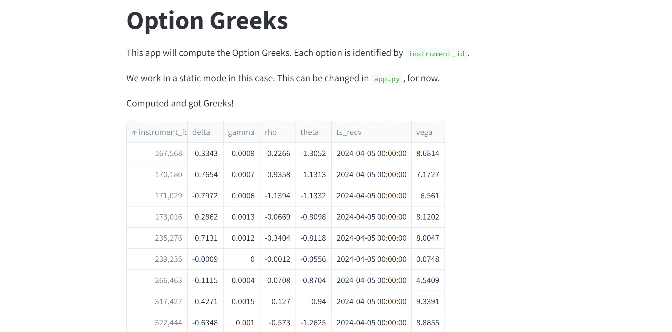
You can find the sources to obtain this dashboard in our public GitHub repository.

Pathway has a unified engine capable of processing both static and streaming data, making it easy to transition from one mode to the other. You can easily make the book orders dynamic by updating the input connector ConnectorSubject (MBP1Subject) to simulate real-time data streaming by adding a time.sleep() function call after each next call. This small modification introduces a delay between data points, emulating the arrival of new data over time. The updated source is available in our public GitHub repository.

In this case, Pathway will update the results every time the input changes, at the reception of new data point from the mbp-1 data for example.

Furthermore, you can use Databento live APIs to obtain the market live data for the book orders and have the option Greeks updated in real-time as the live data is ingested. This way, you can make full use of the streaming mode.

Congratulations! You now are able to compute the implied volatility and the option Greeks using Databento to extract the historical market data and Pathway to process it.

Pathway is a Python data processing framework for analytics and AI pipelines over data streams. It’s the ideal solution for real-time processing use cases like computing the option Greeks. Pathway comes with an easy-to-use Python API, syntax that is simple and intuitive, and you can use the same code for both batch and streaming processing. Pathway is powered by a scalable Rust engine based on Differential Dataflow and performing incremental computation.

Build a fast, real-time stock screener in Python

May 08, 2025

Download and merge PCAPs with Databento for market replay

Roman Bansal, Guest author

May 07, 2025

Getting queue position from L2 and order book data

February 26, 2025

Computing the option Greeks using Pathway and Databento

Related Posts

Build a fast, real-time stock screener in Python

Download and merge PCAPs with Databento for market replay

Getting queue position from L2 and order book data