Building high-frequency trading signals in Python with Databento and sklearn

This is a simple example that demonstrates how to build high-frequency trading signals in Python, using order book and market depth data from Databento together with machine learning models from sklearn.

For this example, we'll use the E-mini S&P 500 futures (ES) contract, using Databento. Here's what you need to get started:

• Dataset ID. ES is traded on CME Globex. We'll fetch its data from CME's primary feed, MDP 3.0, i.e. dataset='GLBX.MDP3'.
• Format and granularity (schema) of data desired. We need 10 levels of market depth. This can be specified with schema='mbp-10'.
• Input symbology system. We'll use the lead month contract, which can be specified with continuous contract symbology orstype_in='continuous'
• Symbol. This would be symbols=['ES.n.0']. Keep in mind that continuous symbols are pegged to the original symbol and simply returns its original prices without any adjustments. If you prefer to work with the raw symbols, you could use stype_in='raw_symbol' and symbols=['ESZ3'] instead to get an identical result, but this would be tedious if your analysis spans over multiple rollovers.

import databento as db


client = db.Historical('YOUR_API_KEY')

# Get 10 levels of ES lead month
data = client.timeseries.get_range(
    dataset='GLBX.MDP3',
    schema='mbp-10',
    start="2023-12-06T14:30",
    end="2023-12-06T20:30",
    symbols=['ES.n.0'],
    stype_in='continuous',
)
df = data.to_df()

We’ll build our model in trade space only to reduce the computational time, but you can do the same analysis on a different event space or subsampling interval.

Likewise, we’ll forecast returns 500 trades out. This is a simplification and you may want to try a different target. In practice, trades may be clustered so there could be no time to act on a prediction that’s 500 trades out, or your strategy may be constructed in a way that can’t monetize trade events with irregular arrival times.

# Filter out trades only
df = df[df.action == 'T']

# Get midprice returns with a forward markout of 500 trades
df['mid'] = (df['bid_px_00'] + df['ask_px_00'])/2
df['ret_500t'] = df['mid'].shift(-500) - df['mid']

df = df.dropna()

We’ll construct two features, the top-of-book skew and order imbalance on the top 10 levels of the book.

Book imbalance, sometimes called skew, is heavily explored in academic publications on order book forecasting and also used widely by practitioners. This is usually defined as the imbalance in aggregate depth between bid and ask sides of the book. Others may call this book pressure. At some firms, these three terms refer to slightly different variations of the same concept.

Order imbalance is similar to skew, except we’ll construct it from the quantity of orders at each price level instead of the aggregate depth. This will help us demonstrate the marginal value-add of features based on order book data. Databento’s MBP-10 schema is a hybrid between MBP with limited depth (sometimes called “L2”) and order-by-order data (sometimes called “L3”), in that it conveniently includes the order count at each price level. This is denoted by side_ct_xx, so for example bid_ct_00 represents the number of orders at the best bid.

import numpy as np

# Depth imbalance on top level ('skew')
df['skew'] = np.log(df.bid_sz_00) - np.log(df.ask_sz_00)

# Order imbalance on top ten levels ('imbalance')
df['imbalance'] = np.log(df[list(df.filter(regex='bid_ct_0[0-9]'))].sum(axis=1)) - \
    np.log(df[list(df.filter(regex='ask_ct_0[0-9]'))].sum(axis=1))

Divide the data into an in-sample and out-of-sample set.

split = int(0.66 * len(df))
split -= split % 100
df_in = df.iloc[:split]
df_out = df.iloc[split:]

We’ll construct a simple trading signal based on these two features.

First, we’ll check the collinearity between our features as well as their correlations against the target.

corr = df_in[['skew', 'imbalance', 'ret_500t']].corr()
print(corr.where(np.triu(np.ones(corr.shape)).astype(bool)))

           skew  imbalance  ret_500t
skew        1.0   0.474489  0.108694
imbalance   NaN   1.000000  0.065495
ret_500t    NaN        NaN  1.000000

As seen here, our order imbalance feature has only moderate correlation against the simple top-of-book skew. Both have some predictive value against short-term future returns; in a low signal-to-noise ratio environment like order book data, it’s common to see useful features like this with R² ≈ 0.01.

Next, we’ll train our model on these two features. sklearn provides various regression models with a simple API. We’ll fit a simple linear regression on our in-sample data and then forecast on our out-of-sample set.

from sklearn.linear_model import LinearRegression

reg = LinearRegression(fit_intercept=False, positive=True)

reg.fit(df_in[['skew']], df_in['ret_500t'])
pred_skew = reg.predict(df_out[['skew']])

reg.fit(df_in[['imbalance']], df_in['ret_500t'])
pred_imbalance = reg.predict(df_out[['imbalance']])

reg.fit(df_in[['skew', 'imbalance']], df_in['ret_500t'])
pred_combined = reg.predict(df_out[['skew', 'imbalance']])

You can easily swap in other models, which can be more appropriate especially as you have more features and nonlinear interactions. For example, uncomment the following four lines to use histogram-based, gradient-boosted trees, similar to LightGBM.

# from sklearn.ensemble import HistGradientBoostingRegressor


# reg = HistGradientBoostingRegressor()
# reg.fit(df_in[['skew', 'imbalance']], df_in['ret_500t'])
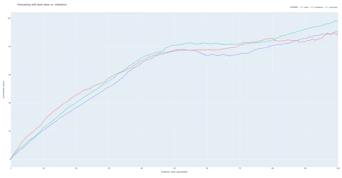
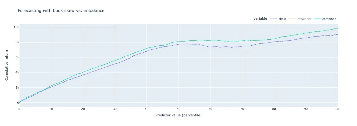
# pred_combined = reg.predict(df_out[['skew', 'imbalance']])

We can compare the distribution of our target against that of each predictor by cumulating the target over sorted values of the predictor. A good signal should exhibit a smoothly increasing curve.

import pandas as pd
import plotly
import plotly.express as px
import plotly.io as pio

# pio.renderers.default = 'notebook'
# pio.renderers.default = 'iframe'

pct = np.arange(0, 100, step=100/len(df_out))

def get_cumulative_markout_pnl(pred):
    df_pnl = pd.DataFrame({'pred': pred, 'ret_500t': df_out['ret_500t'].values})
    df_pnl.loc[df_pnl['pred'] < 0, 'ret_500t'] *= -1
    df_pnl = df_pnl.sort_values(by='pred')
    return df_pnl['ret_500t'].cumsum().values
    
results = pd.DataFrame({
    'pct': pct,
    'skew': get_cumulative_markout_pnl(pred_skew),
    'imbalance': get_cumulative_markout_pnl(pred_imbalance),
    'combined': get_cumulative_markout_pnl(pred_combined),
})

fig = px.line(
    results, x='pct', y=['skew', 'imbalance', 'combined'],
    title='Forecasting with book skew vs. imbalance',
    labels={'pct': 'Predictor value (percentile)'},
)

fig.update_yaxes(title_text='Cumulative return')

fig.update_layout(legend=dict(
    orientation="h",
    yanchor="bottom",
    y=1.02,
    xanchor="right",
    x=1
))

fig.show()

You’ll see that the prediction model based on the order imbalance alone achieves similar performance compared to the one based on top-of-book skew. The combined signal using both features consistently outperforms the top-of-book skew on its own:

You can get this entire example as a single file on GitHub here.