Getting futures tick sizes and notional tick values in Python with Databento

Handling tick sizes and values is tedious, and one of the challenges of trading futures systematically.
While other asset classes like equities and FX are usually traded in dollar units with at most a handful of tick size regimes (e.g. Rule 612, Tick Size Pilot) that can be hardcoded, futures instruments have contract multipliers, variable tick sizes, and display styles that vary from one product to another.
This tutorial shows how you can programmatically extract the tick sizes and notional tick values of futures and options on futures instruments.
We’ll also be doing this to incredible speed and scale, demonstrating how you can extract the tick sizes and values of nearly 800,000 instruments across 6 exchanges (CME, CBOT, NYMEX, COMEX, ICE, Endex) in only around 10 seconds, including the time it takes for data transfer over a regular WiFi connection.
We’ll be doing this in pure Python with Databento.
Most futures instruments trade on CME, so we’ll start with CME and then extend our tutorial to other venues.
There are three ways to get the tick size and value on CME.
From the CME Product Slate, find the product that you’re looking for. Then, head to Contract Specs > Minimum Price Fluctuation. For example, you can find the tick size of ES here.
Many clearing firms and brokers also provide an abridged list of this, which may be easier to use, but tend to be limited only to the 20 to 100 most liquid futures outrights.
In any case, this approach is not recommended for systematic use:
- Many products have specs that are hard to parse. Because the specs are not written in a machine-readable, consistent manner, it’s error-prone to use this.
- It’s hard to determine the tick sizes of non-outright instruments, like spreads, options, user-defined instruments, etc.
- It’s hard to handle instruments with variable tick sizes.
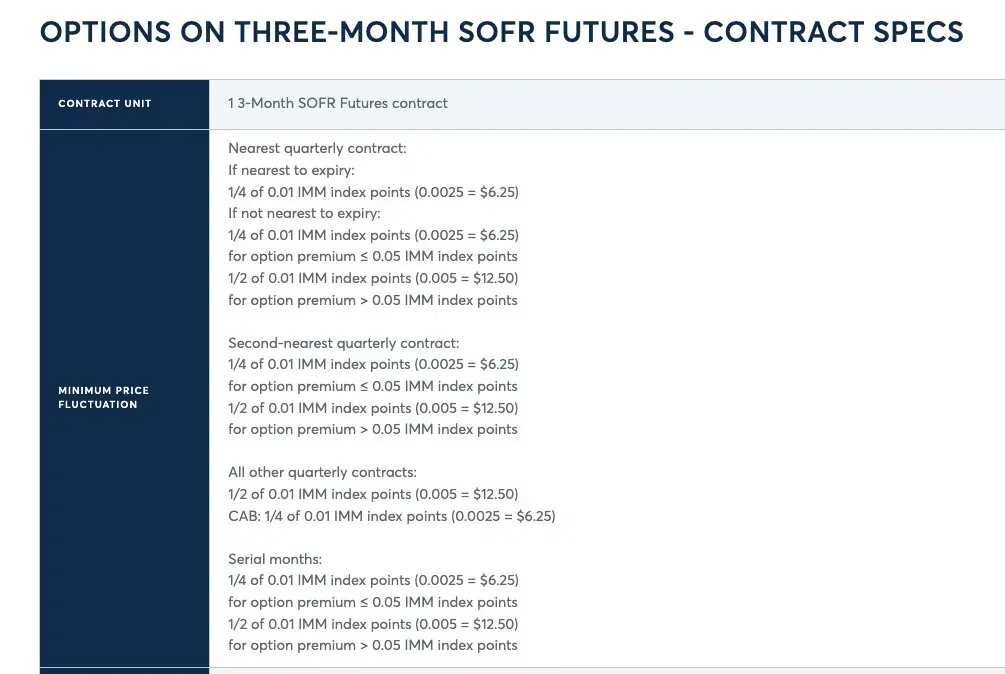
Below is an example description of SOFR tick size and value: Not machine-readable.

The biggest downsides of this are that the API is cumbersome to set up from an administrative standpoint; it’s not performant, and it’s only updated at 7 minute intervals. There’s one upside that this API covers two other major venues—BrokerTec and EBS.
For most users, this is the recommended approach and the one we’ll show in this tutorial.
Raw security definitions can be obtained through the exchange’s direct feed (CME MDP 3.0, ICE iMpact, etc.). CME, for instance, also uploads these in file format to their FTP server—if you wish to use these secdef files, you may follow this GitHub tutorial instead.
An easier way to obtain security definitions is through Databento, which provides them in a normalized format and called instrument definitions. (We chose this name because our definitions generalize across both securities and derivatives, whereas CME’s naming is an unfortunate inheritance of the Security Definition <d> message in the FIX protocol.)
Databento’s instrument definitions are much easier to use than the raw secdefs; they’re also normalized across multiple venues and asset classes, and provided across a very fast API.
The tick size is simply tag 969-MinPriceIncrement. On Databento’s instrument definitions data, this is min_price_increment.
Here’s an example using this together with top of book (MBP-1) data to determine the average spread size:
import databento as db


client = db.Historical()

get_data_df = lambda schema: client.timeseries.get_range(
    dataset="GLBX.MDP3",
    schema=schema,
    symbols=["6AU4"],
    start="2024-07-08",
    end="2024-07-09",
).to_df()

df = get_data_df("mbp-1")
df_def = get_data_df("definition")

spread = (df["ask_px_00"] - df["bid_px_00"]) / df_def["min_price_increment"].iloc[0]
print(spread.mean())
1.0728872573829422
As expected, on the lead month contract of a liquid instrument like 6A, the spread is usually very close to 1 tick wide.
If you’re getting the notional tick value from security definitions, you’ll need these fields:
- tag 207-SecurityExchange
- tag 969-MinPriceIncrement
- tag 1147-UnitofMeasureQty
- tag 9787-DisplayFactor
Databento already handles scaling of the display factor for you, so you’ll only need the first three. As such, the tick value is simply min_price_increment multiplied by unit_of_measure_qty:
import databento as db


client = db.Historical()

data = client.timeseries.get_range(
    dataset="GLBX.MDP3",
    schema="definition",
    symbols="ALL_SYMBOLS",
    start="2024-07-08",
    end="2024-07-09",
)

df = data.to_df()

df["tick_value"] = df["min_price_increment"] * df["unit_of_measure_qty"]
On CBOT, where most US treasury products like ZN and ags like ZC are traded, unit_of_measure_qty is usually quoted in cents.
So you could condition on exchange and scale the tick value by 0.01 if it’s on XCBT :
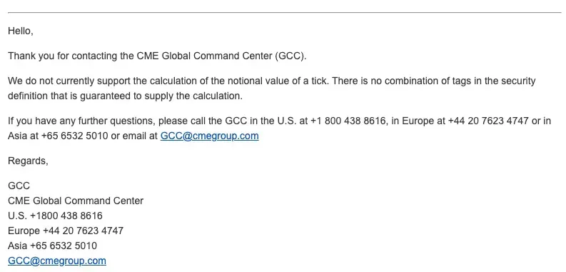
df.loc[df["exchange"] == "XCBT", "tick_value"] *= 0.01Despite this formula working almost all of the time, CME provides no hard guarantee that it is correct. Hence, for all CME exchanges, we recommend using this approach as a first pass and then making a second pass by hand for instruments that you actually trade.

If you paid close attention to the available fields, you’ll notice there’s an additional field called min_price_increment_amount. This is reserved for tag 1146-MinPriceIncrementAmount.
It’s tempting to infer from the field name that this provides the notional tick value for you directly, but as of the time of this writing (Sep 9, 2024), this field is still reserved for future purposes and should not be used.
If you’re switching over to Databento from another data provider, it may strike you as unusual that our instrument definitions data is usually timestamped twice, and down to the nanosecond:
In [1]: df[(df[["min_price_increment"]] != 0).all(axis=1)][["ts_event", "raw_symbol", "min_price_increment"]].dropna()
Out[1]:
                                                               ts_event         raw_symbol  min_price_increment
ts_recv
2024-07-08 00:00:00+00:00              2024-07-07 11:05:11.714000+00:00        A8IU5-A8IV5            0.0000100
2024-07-08 00:00:00+00:00              2024-07-07 11:06:21.051000+00:00             W0N416            0.0010000
2024-07-08 00:00:00+00:00              2024-07-07 11:03:42.455000+00:00       NKWU4 P33200            1.0000000
2024-07-08 00:00:00+00:00              2024-07-07 11:02:27.878000+00:00        OHV4 P24900            0.0001000
2024-07-08 00:00:00+00:00              2024-07-07 11:01:22.171000+00:00         1RQ4 P2220            0.0000100
...                                                                 ...                ...                  ...
2024-07-08 23:51:04.091922032+00:00 2024-07-08 23:51:04.091664899+00:00  UD:T$: SG 2519297            0.0078125
2024-07-08 23:52:42.962625749+00:00 2024-07-08 23:52:42.962023489+00:00  UD:CY: VT 2519305            0.1250000
2024-07-08 23:52:48.935944762+00:00 2024-07-08 23:52:48.935242185+00:00  UD:2U: GN 2519306            0.0005000
2024-07-08 23:54:21.183295894+00:00 2024-07-08 23:54:21.182618265+00:00  UD:1Y: VT 2519314            0.1000000
2024-07-08 23:57:39.820505383+00:00 2024-07-08 23:57:39.819863823+00:00  UD:1Y: VT 2519342            0.1000000
You’ll also notice that we fetched the instrument definitions using the timeseries API method. This is property is called point-in-time data—meaning, data that’s timestamped and ordered as if it had arrived in real-time.
Virtually every other normalized data provider only gives you a cumulative or daily snapshot of listed instruments, which loses this property.
There are important considerations for why you should handle instrument definitions, including attributes like tick sizes and notional tick values, in a point-in-time manner:
- The exchange may change the tick size at any time. A notable example is how KRX changed the contract sizes of KOSPI-200 derivatives on March 27, 2017.
- The tick size may also be variable based on predetermined rules. See for example the
tick_rulefield in Databento’s instrument definitions, which encodestag 6350-TickRuleand the VTT codes found here.
Databento makes it easy for you to reuse your code for any trading venue. This includes how you handle instrument definitions. For example, to get instrument definitions of ICE Europe instead, you just need to swap in dataset="IFEU.IMPACT" .
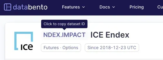
You can find these dataset IDs using the metadata.list_datasets API method or from the dataset specifications page on Databento’s website:

Now, we can stitch everything we’ve learned so far together and get the tick sizes of three trading venues at:
import databento as db
import pandas as pd


client = db.Historical()

def get_definitions(dataset):

    return client.timeseries.get_range(
        dataset=dataset,
        schema="definition",
        symbols="ALL_SYMBOLS",
        start="2024-07-08",
        end="2024-07-09",
    ).to_df()

df_cme = get_definitions("GLBX.MDP3")
df_ice = get_definitions("IFEU.IMPACT")
df_endex = get_definitions("NDEX.IMPACT")
df = pd.concat([df_cme, df_ice, df_endex])

df["tick_size"] = df["min_price_increment"]
df["tick_value"] = df["min_price_increment"] * df["unit_of_measure_qty"]
df.loc[df["exchange"] == "XCBT", "tick_value"] *= 0.01

print(df[(df[["tick_size"]] != 0).all(axis=1)][["raw_symbol", "tick_size", "tick_value"]].dropna())
raw_symbol tick_size tick_value ts_recv 2024-07-08 00:00:00+00:00 W0N416 0.00100 1.00 2024-07-08 00:00:00+00:00 NKWU4 P33200 1.00000 500.00 2024-07-08 00:00:00+00:00 OHV4 P24900 0.00010 4.20 2024-07-08 00:00:00+00:00 1RQ4 P2220 0.00001 1.00 2024-07-08 00:00:00+00:00 RAG5 P15000 0.00010 4.20 ... ... ... ... 2024-07-08 00:00:00+00:00 DIF 89 7813548 0.01000 0.01 2024-07-08 00:00:00+00:00 DIF 89 7813549 0.01000 0.01 2024-07-08 00:00:00+00:00 DFB 89 7813550 0.01000 0.01 2024-07-08 00:00:00+00:00 DGA 89 7813551 0.01000 0.01 2024-07-08 00:00:00+00:00 DGB 89 7813552 0.01000 0.01 [447114 rows x 3 columns]
This example runs in 11.9 seconds across 773,485 instruments—about half are user-defined instruments or other instrument types with undefined tick sizes or values—over a regular internet connection.
