Downsampling pricing data into bars with Python and Polars

The following article was written by our customer Nelson Griffiths, Engineering and Machine Learning Lead at Double River Investments, a quantitative investment manager focusing on global equity markets, utilizing fundamental, technical, and alternative data. Nelson has been using Databento for several months and was happy to share some common ways our users can aggregate and transform their pricing data. We were excited to collaborate with Nelson and see how he's been using our data. In this guest post, he demonstrates how to downsample price data with Python and Polars.

There are a lot of ways to downsample granular market data into useful price bars. The most common of these ways is to sample by time, calculating an OHLCV bar for each second, minute, hour, or day. In some respects, this is a great way to aggregate bars. From a human perspective, it is easy to understand and measure changes in value over set periods of time. However, there are other useful ways to downsample and aggregate this data to provide more information-dense price bars to trading algorithms. All of the strategies I am going to review today can be found in the book Advances in Financial Machine Learning by Marcos Lopez De Prado.

We are going to walk through how to get data that comes from the "trades" schema from Databento's Nasdaq TotalView-ITCH dataset, to calculate two types of price bars: Standard Time Bars and Tick Bars, and understand the differences between each of them.

In a follow-up post, we will look at two other types of pricing bars that contain different types of information:

• Volume Bars
• Dollar Bars

One of my favorite parts of Databento is their attention to performance. In that same line of thinking, we will be going through these exercises using Polars, a DataFrame library written in Rust, as opposed to the very popular Pandas library. This is due to a few reasons:  

• Memory: When we are aggregating huge datasets, being memory efficient is important. And Polars is much better at being memory efficient with data than Pandas.  
• Speed: We will see a huge speed boost using Polars as opposed to Pandas.  
• Type Safety: Polars adheres to a stricter typing system minimizing the potential for errors.

I will defer to other blog posts if you want to read more about the comparison between the two libraries. For my purposes, I will simply state that I believe Polars to be a better option for dealing with the data provided by Databento.

We will go ahead and pull some data from Databento using the Python API. We will grab data for 4 securities over a month time period from the trades schema and load the data into Polars using the code snippet below:

import polars as pl
import databento as db
import datetime as dt

start_time = dt.datetime(2024, 2, 12, 9, 30, 0, 0,
pytz.timezone("US/Eastern"))
end_time = dt.datetime(2024, 3, 12, 16, 0, 0, 0,
pytz.timezone("US/Eastern"))

client = db.Historical() # Either pass your API key here or set your ENV variable.
dbn = client.timeseries.get_range(
    "XNAS.ITCH",
    start_time,
    end_time,
    symbols=["AAPL", "MSFT", "AMZN", "TQQQ"],
    schema="trades"
) # This will cost ~5 dollars.

# Make the dataframe lazy for future ops
df = pl.from_pandas(dbn.to_df().reset_index()).lazy()

We will do a few small things to make the dataset more manageable for our purposes. First, we are going to trim the data down from all columns to just the data we need. We will then change the types of some of our columns so that we are not working with strings. Then for readability, we will convert our UTC date-times to US/Eastern time to line up with the NYSE market hours.  

Here is a quick look at what our data looks like before making any changes:

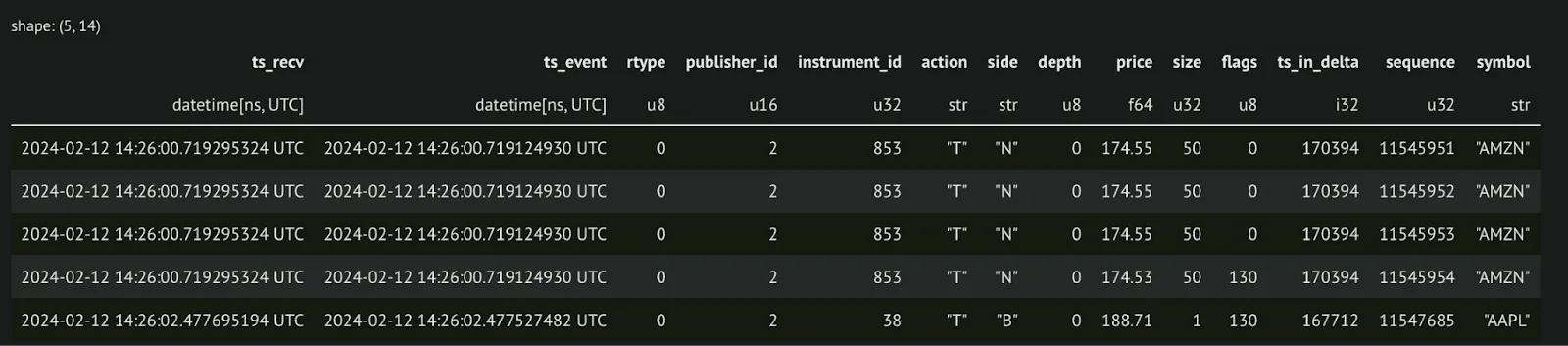
Here's our code to make changes to our data:

df = (
    df.select(
        # We could also set this to pl.Categorical
        pl.col("symbol").cast(pl.Enum(["AAPL", "AMZN", "MSFT", "TQQQ"])),
        pl.col("ts_event").dt.convert_time_zone("US/Eastern"),
        "price",
        "size",
    )
    .sort("symbol", "ts_event")
)

And our resulting data:

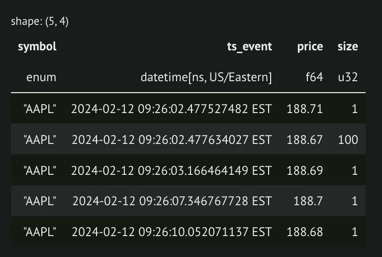
We will start by writing a function that will aggregate our trade data into standard time bars. Below is a function that can take our trades and aggregate them at any time level we would like.

def standard_bars(
        df: FrameType,
        timestamp_col: str = "ts_event",
        price_col: str = "price",
        size_col: str = "size",
        symbol_col: str = "symbol",
        bar_size: str = "1m",
    ):
        ohlcv = (
            # We won't consider any rows where a trade may not have a price for some reason.
            df.drop_nulls(subset=price_col)
            # We can use polars' truncate function to set our time column to set intervals

.with_columns(pl.col(timestamp_col).dt.truncate(bar_size))
            # This group by will group by our time groups and columns so this can be applied to time series with multiple symbols
            
            .group_by(timestamp_col, symbol_col)
            # Calculate our OHLCV columns and include a count of the number of trades in a group
            .agg(
                pl.first(price_col).alias("open"),
                pl.max(price_col).alias("high"),
                pl.min(price_col).alias("low"),
                pl.last(price_col).alias("close"),
                (
                    (pl.col(size_col) * pl.col(price_col)).sum() / pl.col(size_col).sum()
                ).alias("vwap"),
                pl.sum(size_col).alias("volume"),
                pl.len().alias("n_trades"),
            )
            .sort(timestamp_col)
        )
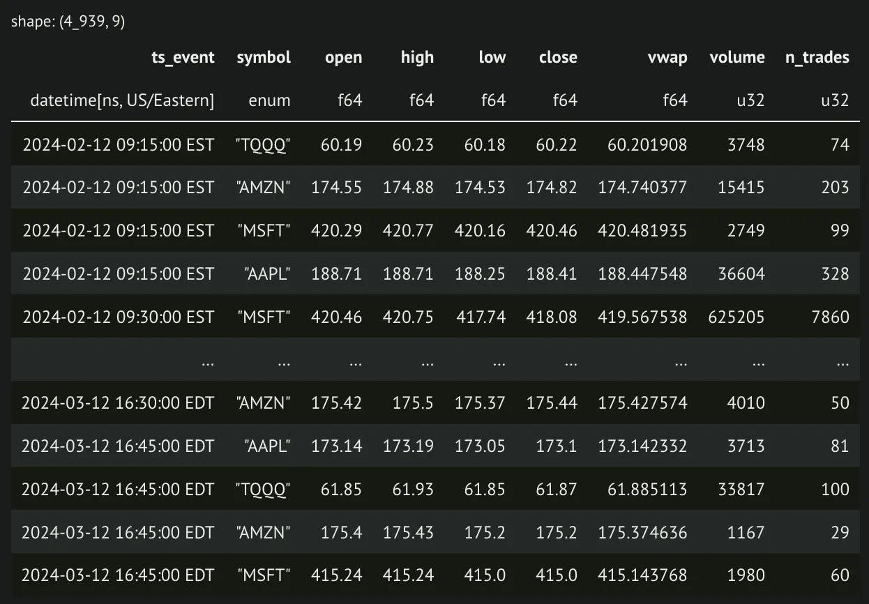
        return ohlcv

With this function we can pass any string representing time to our bar size to aggregate our OHLCV bars. For example, we can pass '1s' to get 1-second bars, or '15m' to get 15-minute bars. Let's apply this to our data.

standard_bars(df, bar_size="15m").collect()

And the resulting data:

One alternative to the standard time bars is to use bars aggregated by ticks, or trades. One advantage of this is that we change from a constant time interval sampling to a sampling focused on when activity is happening in the market. The way we do this is by sampling a bar every time a certain number of ticks occur for a security. We will make a few decisions while calculating this for simplicity.  

1. We will not allow bars to cross over between market sessions.  
2. We will have a constant bar size across all securities.

Here is our function to calculate tick bars along with a helper function we will use to make the OHLCV calculations:

def _ohlcv_expr(timestamp_col: str, price_col: str, size_col: str) -> list[pl.Expr]:
    return [
        pl.first(timestamp_col).name.prefix("begin_"),
        pl.last(timestamp_col).name.prefix("end_"),
        pl.first(price_col).alias("open"),
        pl.max(price_col).alias("high"),
        pl.min(price_col).alias("low"),
        pl.last(price_col).alias("close"),
        ((pl.col(size_col) * pl.col(price_col)).sum() / pl.col(size_col).sum()).alias(
            "vwap"
        ),
        pl.sum(size_col).alias("volume"),
        pl.len().alias("n_trades"),
    ]


def tick_bars(
    df: FrameType,
    timestamp_col: str = "ts_event",
    price_col: str = "price",
    size_col: str = "size",
    symbol_col: str = "symbol",
    bar_size: int = 100,
):
    ohlcv = (
        # We will ignore trades where there is no price for any reason.
        df.drop_nulls(subset=price_col)
        # We need to ensure we are sorted
        .sort(timestamp_col)
        # Create an indicator of each market session. Date in this case.
        .with_columns(pl.col(timestamp_col).dt.date().alias("__date"))
    )
    ohlcv = ohlcv.with_columns(
        (
            # Get a rolling tick count for each symbol on each date
            # Divide that rolling count by our group size. 
            ((pl.col(symbol_col).cum_count()).over(symbol_col, "__date") - 1)
            // bar_size
        ).alias(
            "__tick_group",
        )
    )
    ohlcv = (
        # Group by symbols, dates, and our tick group calculated above.
        ohlcv.group_by("__tick_group", symbol_col, "__date")
        .agg(_ohlcv_expr(timestamp_col, price_col, size_col))
        .drop("__tick_group", "__date")
        .sort(f"begin_{timestamp_col}")
    )
    return ohlcv

And a look at our output: tick_bars(df, bar_size=200).collect()

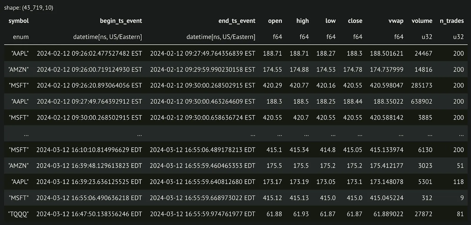
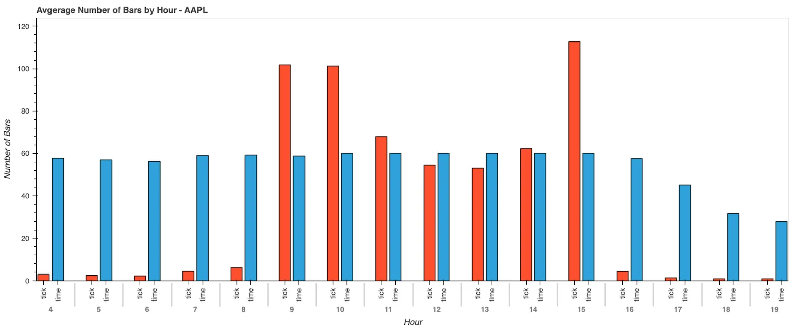
Now that we have calculated two different kinds of bars, let’s look at the difference between them. We are going to graph the average number of bars for a single security, AAPL, across the last month of data. What we find is that, as expected, we get more tick bars during periods where we expect a lot of information to be coming in, and fewer bars during times when we expect very little is happening.

We have explored two different ways to downsample pricing data from Databento to create pricing bars. While we have shown that tick bars have some properties that in some cases are more desirable than standard time bars, they are far from perfect. They suffer from some problems of their own. In a future post, we will look at other types of bars that we can calculate that may improve upon the properties of tick bars to provide a more robust set of information for algorithms to learn from and how we can harness the power of Rust to do so efficiently.