Algorithmic trading guide: high-frequency, liquidity-taking strategy

In an earlier guide, we showed you how to build an algorithmic trading strategy with a model-based (machine learning) alpha in Python with Databento and sklearn.

In this guide, we'll walk you through how to build a rule-based algorithmic trading strategy instead. We'll also show you how you can compute trading metrics like PnL online with Databento's real-time feed. This example is adaptable to high-frequency trading (HFT) and mid-frequency trading scenarios.

Before breaking down the strategy, let's explain some terminology:

Feature: Any kind of basic independent variable that's thought to have some predictive value. This follows machine learning nomenclature; others may refer to this as a predictor or regressor in a statistical or econometric setting.

Trading rule: A hardcoded trading decision. For example, "If there's only one order left at the best offer, lift the offer; if there is only one order left at the best bid, hit the bid." A trading rule may be a hardcoded trading decision taken when a feature value exceeds a certain threshold.

Rule-based strategy: A strategy that's based on trading rules instead of model-based alphas.

Liquidity-taking strategy: A strategy that takes liquidity by crossing the spread with aggressive or marketable orders.

High-frequency strategy: A strategy characterized by a large number of trades. There's no public consensus on what this means, but such strategies will usually show high directional turnover, at least 20 bps ADV, and small maximum position. Importantly, low latency and short holding period are not necessary conditions, but in practice, most such strategies exhibit sharp decay in PnL up to 15 microseconds wire-to-wire.

Mid-frequency strategy: There's also no public convention on this term, but we'll use it to refer to a relaxation of the low latency and directional turnover conditions as compared to a high-frequency strategy; a mid-frequency strategy will usually have intraday directional turnover in the order of hours for liquid instruments.

Now that we have a few key terms defined, let's dive into the strategy.

One of the simplest types of book feature is called the book skew, which is the imbalance between resting bid depth $(v_b)$ and resting ask depth $(v_a)$ at the top of the book. We can formulate this as some difference between $v_b$ and $v_a$ . It's convenient to scale these by their order of magnitude, so we take their log differences instead.

Notice that we picked this ordering simply because it's useful to formulate features such that positive values imply that we expect prices to increase, making debugging your strategy easier. Intuitively, we expect higher bid depth to indicate higher buy demand and, hence, higher prices.

We can introduce a trading rule that buys when this feature exceeds some skew threshold k and sells when it goes below some threshold -k.

While there are some practical advantages to trading larger clips for a liquidity-taking strategy, we'll start with a constant trade size equal to the minimum order quantity to minimize slippage and market impact considerations.

The minimum order quantity depends on the trading platform or market that you're on. For this sample strategy, we'll use the E-mini S&P 500 (ES) futures contract as an example and trade in clips of 1 contract.

Due to its volume, this strategy will be very sensitive to commissions, so we'll include commissions on the estimated PnL. You can find these commissions here.

This strategy is convenient because you don't have to worry about complex order and position state management. You just let it build up whatever maximum position you want. You'll eventually get out of position because we expect buys and sells to be symmetrically distributed in the long run. However, you might need more margin to build up arbitrarily large positions, so we'll specify a maximum position of 10 contracts for proof of concept.

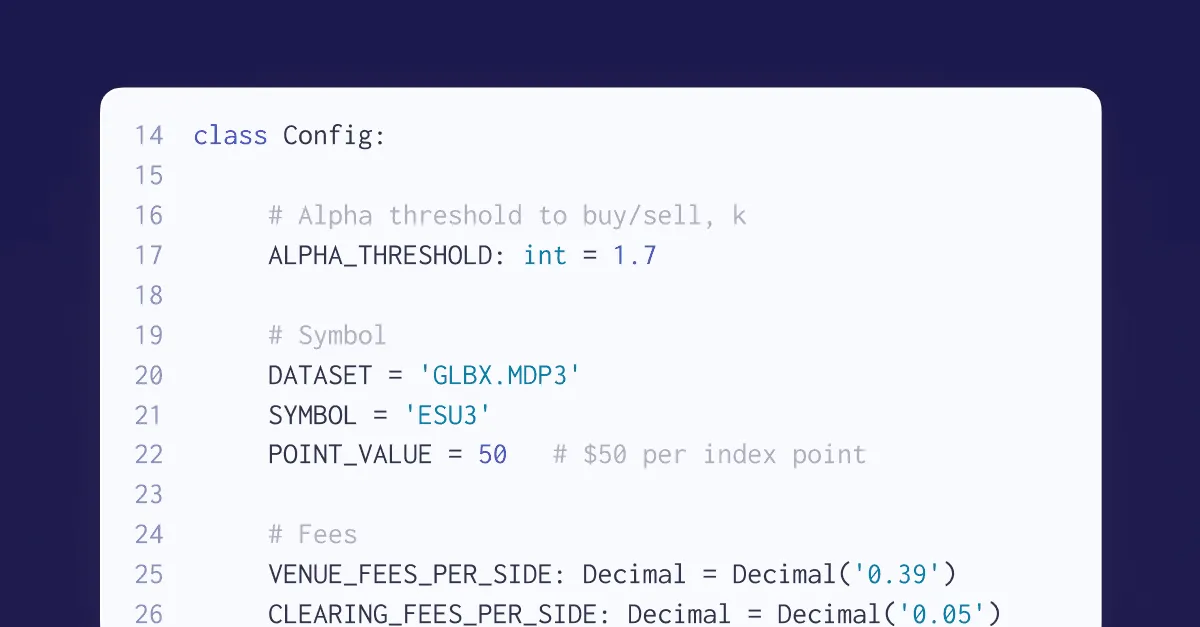
Here are the parameters we have so far. We're using the instrument with raw symbol ESU3 (which is the September expiring contract). You'll need to substitute this with your desired symbol.

import math
from pprint import pprint
from dataclasses import dataclass, field
from decimal import Decimal
from typing import Optional, List

import pandas as pd
import databento as db


@dataclass(frozen=True)
class Config:
    # Databento API Key
    api_key: Optional[str] = None  # "YOUR_API_KEY"

    # Alpha threshold to buy/sell, k
    skew_threshold: float = 1.7

    # Databento dataset
    dataset: str = "GLBX.MDP3"

    # Instrument information
    symbol: str = "ES.c.0"
    stype_in: str = "continuous"
    point_value: Decimal = Decimal("50")  # $50 per index point

    # Fees
    venue_fees_per_side: Decimal = Decimal("0.39")
    clearing_fees_per_side: Decimal = Decimal("0.05")

    @property
    def fees_per_side(self) -> Decimal:
        return self.venue_fees_per_side + self.clearing_fees_per_side

    # Position limit
    position_max: int = 10

Since we're only simulating liquidity-taking at minimum size, our mbp-1 schema, which represents the top-of-book best bid and ask, is sufficient.

To simplify this example, we'll assume zero round-trip latency for any orders placed. This is unrealistic as this type of strategy will be extremely sensitive to latency, but allows us to demonstrate how to implement a simple, online calculation of PnL for our real-time trading simulation.

An online algorithm like this is beneficial as the runtime and memory requirements do not increase with the number of data points used or number of orders placed in the simulation.

@dataclass
class Strategy:
    # Static configuration
    config: Config

    # Current position, in contract units
    position: int = 0
    # Number of long contract sides traded
    buy_qty: int = 0
    # Number of short contract sides traded
    sell_qty: int = 0

    # Total realized buy price
    real_total_buy_px: Decimal = Decimal("0")
    # Total realized sell price
    real_total_sell_px: Decimal = Decimal("0")

    # Total buy price to liquidate current position
    theo_total_buy_px: Decimal = Decimal("0")
    # Total sell price to liquidate current position
    theo_total_sell_px: Decimal = Decimal("0")

    # Total fees paid
    fees: Decimal = Decimal("0")

    # List to track results
    results: List[object] = field(default_factory=list)

    def run(self) -> None:
        client = db.Live(self.config.api_key)
        client.subscribe(
            dataset=self.config.dataset,
            schema="mbp-1",
            stype_in=self.config.stype_in,
            symbols=[self.config.symbol],
        )
        for record in client:
            if isinstance(record, db.MBP1Msg):
                self.update(record)

    def update(self, record: db.MBP1Msg) -> None:
        ask_size = record.levels[0].ask_sz
        bid_size = record.levels[0].bid_sz
        ask_price = record.levels[0].ask_px / Decimal("1e9")
        bid_price = record.levels[0].bid_px / Decimal("1e9")

        # Calculate skew feature
        skew = math.log10(bid_size) - math.log10(ask_size)

        # Buy/sell based when skew signal is large
        if (
            skew > self.config.skew_threshold
            and self.position < self.config.position_max
        ):
            self.position += 1
            self.buy_qty += 1
            self.real_total_buy_px += ask_price
            self.fees += self.config.fees_per_side
        elif (
            skew < -self.config.skew_threshold
            and self.position > -self.config.position_max
        ):
            self.position -= 1
            self.sell_qty += 1
            self.real_total_sell_px += bid_price
            self.fees += self.config.fees_per_side

        # Update prices
        # Fill prices are based on BBO with assumed zero latency
        # In practice, fill prices will likely be worse
        if self.position == 0:
            self.theo_total_buy_px = Decimal("0")
            self.theo_total_sell_px = Decimal("0")
        elif self.position > 0:
            self.theo_total_sell_px = bid_price * abs(self.position)
        elif self.position < 0:
            self.theo_total_buy_px = ask_price * abs(self.position)

        # Compute PnL
        theo_pnl = (
            self.config.point_value
            * (
                self.real_total_sell_px
                + self.theo_total_sell_px
                - self.real_total_buy_px
                - self.theo_total_buy_px
            )
            - self.fees
        )

        # Print & store results
        result = {
            "ts_strategy": record.pretty_ts_recv,
            "bid": bid_price,
            "ask": ask_price,
            "skew": skew,
            "position": self.position,
            "trade_ct": self.buy_qty + self.sell_qty,
            "fees": self.fees,
            "pnl": theo_pnl,
        }
        pprint(result)
        self.results.append(result)


if __name__ == "__main__":
    config = Config()
    strategy = Strategy(config=config)
    try:
        strategy.run()
    except KeyboardInterrupt:
        pass
    df = pd.DataFrame.from_records(strategy.results, index="ts_strategy")
    df.to_csv("strategy_log.csv")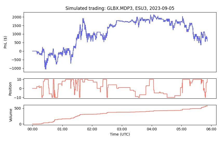

This is a naive strategy to demonstrate the use of Databento and will usually show positive gross PnL before transaction costs and latency, but negative net PnL after. You should not deploy this into production as is.

This implementation uses our simple synchronous client. For production applications, we recommend using our asynchronous client or callback model.

There are various considerations to improve the strategy itself. This strategy only has an entry rule and only takes liquidity; it also has naive inventory management, and it will be sensitive to how the monetization parameter k is selected or optimized. A problem with the book skew is that spoofing may influence extreme values. One possibility is to modify the trading rule and introduce an upper limit as follows:

You can also replace or combine our rule-based signal here with a ML-based alpha, like the one found in the earlier tutorial on Databento's blog.

Finally, recall that we assumed zero delays in order placement and fill. It's also important to incorporate a delay when extending this example.

That's all for this simple liquidity-taking strategy. To learn more, you can check out our docs site, see more examples of our data, or see our client libraries on our GitHub.

This post is for illustrative purposes only and is not intended as investment advice.