How to calculate VWAP in Python with Databento and pandas
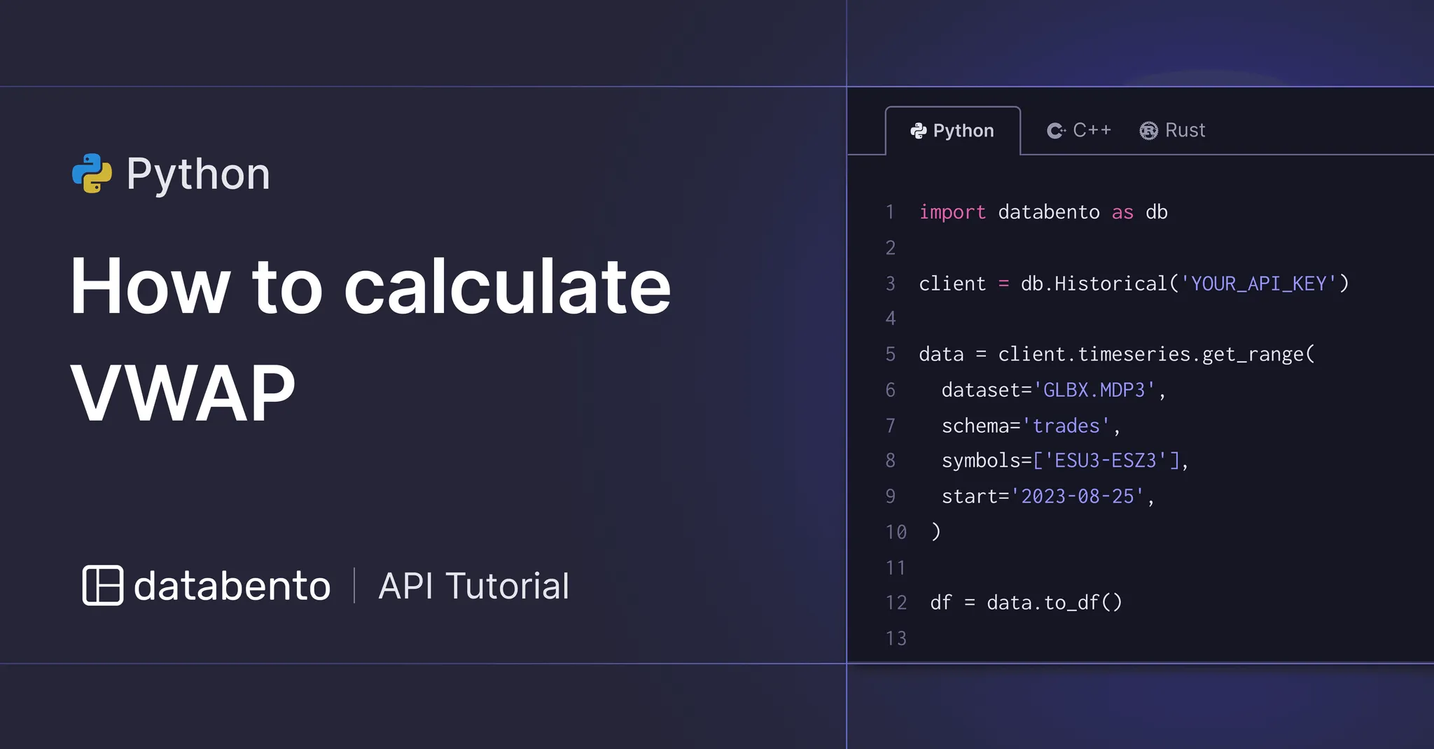
This guide explains the VWAP, its construction and use cases, and how you can compute it quickly in Python with data from Databento.
The volume-weighted price average (VWAP) is a commonly used execution benchmark.
For example, when executing a parent order over a fixed period, the execution quality may be evaluated based on the number of basis points (bps) that the average fill price was better than VWAP in that period.
Since VWAP is widely used by agency execution desks to express execution quality, this creates a self-fulfilling effect where VWAP is an important price level and may be used as a predictive feature, especially at common execution horizons like 1 day.
The formulation of VWAP is simple:
There’s no strict definition that you must use a specific form of price or sampling frequency. So it’s possible to compute VWAP either with OHLCV aggregates or tick-by-tick with last sales (for that matter L1 or time and sales data)
Since Databento supports multiple data formats, also called “schemas”, we can easily demonstrate how to compute VWAP in both ways.
Databento also has built-in support for pandas, which is great for this example because the sum products and elementwise operations in the VWAP formula are easily expressed in pandas with vectorized expressions.
Charting apps often compute VWAP on OHLCV aggregates, say using 1-minute close prices and volumes. These can be obtained from Databento’s ohlcv-1m schema.
We’ll replicate this on NVDA stock prices:
import databento as db


client = db.Historical("YOUR_API_KEY")

data = client.timeseries.get_range(
    dataset="XNAS.ITCH",
    start="2022-09-20",
    symbols=["NVDA"],
    stype_in="raw_symbol",
    schema="ohlcv-1m",
)

# Convert to a DataFrame
ohlcv_data = data.to_df()

# Calculate VWAP using close prices
ohlcv_data["pvt"] = ohlcv_data["close"] * ohlcv_data["volume"]

# Alternatively, calculate VWAP using mean of open, high, close prices
# ohlcv_data["pvt"] = ohlcv_data[["open", "high", "close"]].mean(axis=1) * ohlcv_data["volume"]

ohlcv_data["vwap"] = ohlcv_data["pvt"].cumsum() / ohlcv_data["volume"].cumsum()

print(ohlcv_data[["symbol", "open", "close", "vwap"]])
symbol open close vwap
ts_event
2022-09-20 08:00:00+00:00 NVDA 133.380 133.170 133.170000000
2022-09-20 08:01:00+00:00 NVDA 133.170 133.340 133.232213115
2022-09-20 08:02:00+00:00 NVDA 133.100 133.080 133.199489023
2022-09-20 08:03:00+00:00 NVDA 133.100 133.050 133.161253521
2022-09-20 08:04:00+00:00 NVDA 133.050 133.000 133.152816337
2022-09-20 08:05:00+00:00 NVDA 132.950 132.920 133.151089030
2022-09-20 08:06:00+00:00 NVDA 133.150 133.020 133.150363636
2022-09-20 08:07:00+00:00 NVDA 133.020 132.920 133.131422007
2022-09-20 08:08:00+00:00 NVDA 132.930 132.740 133.076282984
2022-09-20 08:09:00+00:00 NVDA 132.870 132.880 133.059227851
2022-09-20 08:10:00+00:00 NVDA 132.940 132.860 133.053750923 It’s easy to modify the above code to compute VWAP using tick-level trades instead, i.e. with Databento’s trades schema.
There are only two small differences: the trade price is simply found in the price field and the volume is found in the size field:
data = client.timeseries.get_range(
    dataset="XNAS.ITCH",
    start="2022-09-20",
    symbols=["NVDA"],
    stype_in="raw_symbol",
    schema="trades",    # Use tick-by-tick trades instead
)

# Convert to a DataFrame
df = data.to_df()

# Calculate VWAP using close prices
df["pvt"] = df["price"] * df["size"]

df["vwap"] = df["pvt"].cumsum() / df["size"].cumsum()

print(df[["symbol", "price", "vwap"]])
symbol price vwap
ts_recv
2022-09-20 08:00:18.777587048+00:00 NVDA 133.38 133.380000000
2022-09-20 08:00:18.777587048+00:00 NVDA 133.42 133.386666667
2022-09-20 08:00:18.777587048+00:00 NVDA 133.43 133.404000000
2022-09-20 08:00:19.191961847+00:00 NVDA 133.40 133.403200000
2022-09-20 08:00:29.302335850+00:00 NVDA 133.39 133.400645161
... ... ... ...
2022-09-20 23:57:08.376523375+00:00 NVDA 131.54 132.503784836
2022-09-20 23:57:24.638954944+00:00 NVDA 131.68 132.503783783
2022-09-20 23:58:55.036247499+00:00 NVDA 131.60 132.503783668
2022-09-20 23:59:09.753291472+00:00 NVDA 131.56 132.503782462
2022-09-20 23:59:47.114153377+00:00 NVDA 131.53 132.503776864
[101230 rows x 3 columns]This example runs in under 1.8 seconds end-to-end, including extraction of data, on a regular home workstation environment with Databento 0.39.0 and pandas 2.2.2.
Databento is a simpler, faster way to get market data. We’re an official distributor of real-time and historical data for over 40 venues, and provide APIs and other solutions for accessing market data.
Interested to see more examples like this? See Databento’s API documentation.