


This example uses the instrument with raw symbol ESU3. You'll need to substitute this with your desired symbol.
Examples and tutorials
Options
Equity options: Introduction
Options on futures: Introduction
All options with a given underlying
Join options with underlying prices
US equity options volume by venue
Resample US equity options NBBO
Estimate implied volatility
Get symbols for 0DTE options
Daily statistics for equity options
Get end of day option spreads
Historical data
Programmatic batch downloads
Best bid, best offer, and midprice
Custom OHLCV bars from trades
Join schemas on instrument ID
Plot a candlestick chart
Calculate VWAP and RSI
End-of-day pricing and portfolio valuation
Benchmark portfolio performance
Market halts, volatility interrupts, and price bands
Resample OHLCV from 1-minute to 5-minute
Convert DBN to other encoding formats
Request a large number of symbols
Algorithmic trading
A high-frequency liquidity-taking strategy
Build prediction models with machine learning
Execution slippage and markouts
Matching engine latencies
Using messaging rates as a proxy for implied volatility
Mean reversion and portfolio optimization
Pairs trading based on cointegration
Build a real-time stock screener
Core concepts
Venues and datasets
Blue Ocean ATS MEMOIR Depth
Cboe BYX Depth
Cboe BZX Depth
Cboe EDGA Depth
Cboe EDGX Depth
CFE
CME Globex MDP 3.0
Databento US Equities Mini
Databento US Equities Summary
Eurex
European Energy Exchange
ICE Endex
ICE Europe Commodities
ICE Europe Financials
ICE Futures US
IEX TOPS
MEMX MEMOIR Depth
MIAX Pearl Depth of Market
Nasdaq Basic with NLS Plus
Nasdaq TotalView-ITCH
Nasdaq Texas TotalView-ITCH
Nasdaq PSX TotalView-ITCH
NYSE Integrated
NYSE American Integrated
NYSE Arca Integrated
NYSE National Trades and BBO
NYSE Texas Integrated
OPRA
Adjustment factors
Corporate actions
Security master
API Reference
Resources
Release notes
C++
0.62.0 - 2026-07-14
0.61.0 - 2026-07-07
0.60.0 - 2026-06-16
0.59.0 - 2026-06-02
0.58.0 - 2026-05-26
0.57.0 - 2026-05-12
0.56.0 - 2026-05-05
0.55.0 - 2026-04-28
0.54.0 - 2026-04-21
0.53.0 - 2026-04-08
0.52.0 - 2026-03-31
0.51.0 - 2026-03-17
0.50.0 - 2026-03-03
0.49.0 - 2026-02-24
0.48.0 - 2026-02-18
0.47.0 - 2026-02-04
0.46.1 - 2026-01-27
0.46.0 - 2026-01-20
0.45.0 - 2025-12-10
0.44.0 - 2025-11-18
0.43.0 - 2025-10-22
0.42.0 - 2025-08-19
0.41.0 - 2025-08-12
0.40.0 - 2025-07-29
0.39.1 - 2025-07-22
0.39.0 - 2025-07-15
0.38.2 - 2025-07-01
0.38.1 - 2025-06-25
0.38.0 - 2025-06-10
0.37.1 - 2025-06-03
0.37.0 - 2025-06-03
0.36.0 - 2025-05-27
0.35.1 - 2025-05-20
0.35.0 - 2025-05-13
0.34.2 - 2025-05-06
0.34.1 - 2025-04-29
0.34.0 - 2025-04-22
0.33.0 - 2025-04-15
0.32.1 - 2025-04-07
0.32.0 - 2025-04-02
0.31.0 - 2025-03-18
0.30.0 - 2025-02-11
0.29.0 - 2025-02-04
0.28.0 - 2025-01-21
0.27.0 - 2025-01-07
0.26.0 - 2024-12-17
0.25.0 - 2024-11-12
0.24.0 - 2024-10-22
0.23.0 - 2024-09-25
0.22.0 - 2024-08-27
0.21.0 - 2024-07-30
0.20.1 - 2024-07-16
0.20.0 - 2024-07-09
0.19.1 - 2024-06-25
0.19.0 - 2024-06-04
0.18.1 - 2024-05-22
0.18.0 - 2024-05-14
0.17.1 - 2024-04-08
0.17.0 - 2024-04-01
0.16.0 - 2024-03-01
0.15.0 - 2024-01-16
0.14.1 - 2023-12-18
0.14.0 - 2023-11-23
0.13.1 - 2023-10-23
0.13.0 - 2023-09-21
0.12.0 - 2023-08-24
0.11.0 - 2023-08-10
0.10.0 - 2023-07-20
0.9.1 - 2023-07-11
0.9.0 - 2023-06-13
0.8.0 - 2023-05-16
0.7.0 - 2023-04-28
0.6.1 - 2023-03-28
0.6.0 - 2023-03-24
0.5.0 - 2023-03-13
0.4.0 - 2023-03-02
0.3.0 - 2023-01-06
0.2.0 - 2022-12-01
0.1.0 - 2022-11-07
Python
0.81.0 - 2026-07-07
0.80.0 - 2026-06-16
0.79.0 - 2026-06-02
0.78.0 - 2026-05-12
0.77.0 - 2026-04-28
0.76.0 - 2026-04-21
0.75.0 - 2026-04-07
0.74.1 - 2026-03-31
0.74.0 - 2026-03-24
0.73.0 - 2026-03-10
0.72.0 - 2026-02-26
0.71.0 - 2026-02-17
0.70.0 - 2026-01-27
0.69.0 - 2026-01-13
0.68.2 - 2026-01-06
0.68.1 - 2025-12-16
0.68.0 - 2025-12-09
0.67.0 - 2025-12-02
0.66.0 - 2025-11-18
0.65.0 - 2025-11-11
0.64.0 - 2025-09-30
0.63.0 - 2025-09-02
0.62.0 - 2025-08-19
0.61.0 - 2025-08-12
0.60.0 - 2025-08-05
0.59.0 - 2025-07-15
0.58.0 - 2025-07-08
0.57.1 - 2025-06-17
0.57.0 - 2025-06-10
0.56.0 - 2025-06-03
0.55.1 - 2025-06-02
0.55.0 - 2025-05-29
0.54.0 - 2025-05-13
0.53.0 - 2025-04-29
0.52.0 - 2025-04-15
0.51.0 - 2025-04-08
0.50.0 - 2025-03-18
0.49.0 - 2025-03-04
0.48.0 - 2025-01-21
0.47.0 - 2024-12-17
0.46.0 - 2024-12-10
0.45.0 - 2024-11-12
0.44.1 - 2024-10-29
0.44.0 - 2024-10-22
0.43.1 - 2024-10-15
0.43.0 - 2024-10-09
0.42.0 - 2024-09-23
0.41.0 - 2024-09-03
0.40.0 - 2024-08-27
0.39.3 - 2024-08-20
0.39.2 - 2024-08-13
0.39.1 - 2024-08-13
0.39.0 - 2024-07-30
0.38.0 - 2024-07-23
0.37.0 - 2024-07-09
0.36.3 - 2024-07-02
0.36.2 - 2024-06-25
0.36.1 - 2024-06-18
0.36.0 - 2024-06-11
0.35.0 - 2024-06-04
0.34.1 - 2024-05-21
0.34.0 - 2024-05-14
0.33.0 - 2024-04-16
0.32.0 - 2024-04-04
0.31.1 - 2024-03-20
0.31.0 - 2024-03-05
0.30.0 - 2024-02-22
0.29.0 - 2024-02-13
0.28.0 - 2024-02-01
0.27.0 - 2024-01-23
0.26.0 - 2024-01-16
0.25.0 - 2024-01-09
0.24.1 - 2023-12-15
0.24.0 - 2023-11-23
0.23.1 - 2023-11-10
0.23.0 - 2023-10-26
0.22.1 - 2023-10-24
0.22.0 - 2023-10-23
0.21.0 - 2023-10-11
0.20.0 - 2023-09-21
0.19.1 - 2023-09-08
0.19.0 - 2023-08-25
0.18.1 - 2023-08-16
0.18.0 - 2023-08-14
0.17.0 - 2023-08-10
0.16.1 - 2023-08-03
0.16.0 - 2023-07-25
0.15.2 - 2023-07-19
0.15.1 - 2023-07-06
0.15.0 - 2023-07-05
0.14.1 - 2023-06-16
0.14.0 - 2023-06-14
0.13.0 - 2023-06-02
0.12.0 - 2023-05-01
0.11.0 - 2023-04-13
0.10.0 - 2023-04-07
0.9.0 - 2023-03-10
0.8.1 - 2023-03-05
0.8.0 - 2023-03-03
0.7.0 - 2023-01-10
0.6.0 - 2022-12-02
0.5.0 - 2022-11-07
0.4.0 - 2022-09-14
0.3.0 - 2022-08-30
HTTP API
0.36.0 - TBD
0.35.0 - 2025-08-19
0.34.1 - 2025-06-17
0.34.0 - 2025-06-09
0.33.0 - 2024-12-10
0.32.0 - 2024-11-26
0.31.0 - 2024-11-12
0.30.0 - 2024-09-24
0.29.0 - 2024-09-03
0.28.0 - 2024-06-25
0.27.0 - 2024-06-04
0.26.0 - 2024-05-14
0.25.0 - 2024-03-26
0.24.0 - 2024-03-06
0.23.0 - 2024-02-15
0.22.0 - 2024-02-06
0.21.0 - 2024-01-30
0.20.0 - 2024-01-18
0.19.0 - 2023-10-17
0.18.0 - 2023-10-11
0.17.0 - 2023-10-04
0.16.0 - 2023-09-26
0.15.0 - 2023-09-19
0.14.0 - 2023-08-29
0.13.0 - 2023-08-23
0.12.0 - 2023-08-10
0.11.0 - 2023-07-25
0.10.0 - 2023-07-06
0.9.0 - 2023-06-01
0.8.0 - 2023-05-01
0.7.0 - 2023-04-07
0.6.0 - 2023-03-10
0.5.0 - 2023-03-03
0.4.0 - 2022-12-02
0.3.0 - 2022-08-30
0.2.0 - 2021-12-10
0.1.0 - 2021-08-30
Raw API
0.9.1 - TBD
0.9.0 - 2026-04-26
0.7.5 - 2026-02-28
0.7.4 - 2026-02-15
0.7.3 - 2026-02-10
0.7.2 - 2025-12-14
0.7.1 - 2025-11-09
0.7.0 - 2025-10-26
0.6.4 - 2025-09-28
0.6.3 - 2025-09-07
0.6.2 - 2025-08-02
0.6.1 - 2025-06-29
0.6.0 - 2025-05-24
0.5.6 - 2025-04-06
0.5.5 - 2024-12-01
0.5.4 - 2024-10-02
0.5.3 - 2024-10-02
0.5.1 - 2024-07-24
2024-07-20
2024-06-25
0.5.0 - 2024-05-25
0.4.6 - 2024-04-13
0.4.5 - 2024-03-25
0.4.4 - 2024-03-23
0.4.3 - 2024-02-13
0.4.2 - 2024-01-06
0.4.0 - 2023-11-08
0.3.0 - 2023-10-20
0.2.0 - 2023-07-23
0.1.0 - 2023-05-01
Rust
0.55.0 - Upcoming
0.54.0 - 2026-07-07
0.53.0 - 2026-06-02
0.52.0 - 2026-05-26
0.51.0 - 2026-05-12
0.50.0 - 2026-05-05
0.49.0 - 2026-04-29
0.48.0 - 2026-04-21
0.47.0 - 2026-04-15
0.46.0 - 2026-04-07
0.45.0 - 2026-03-31
0.44.0 - 2026-03-17
0.43.0 - 2026-03-04
0.42.0 - 2026-02-24
0.41.0 - 2026-02-18
0.40.0 - 2026-01-27
0.39.0 - 2026-01-20
0.38.0 - 2025-12-16
0.37.0 - 2025-12-09
0.36.0 - 2025-11-19
0.35.0 - 2025-10-22
0.34.1 - 2025-09-30
0.34.0 - 2025-09-23
0.33.1 - 2025-08-26
0.33.0 - 2025-08-19
0.32.0 - 2025-08-12
0.31.0 - 2025-07-30
0.30.0 - 2025-07-22
0.29.0 - 2025-07-15
0.28.0 - 2025-07-01
0.27.1 - 2025-06-25
0.27.0 - 2025-06-10
0.26.2 - 2025-06-03
0.26.1 - 2025-05-30
0.26.0 - 2025-05-28
0.25.0 - 2025-05-13
0.24.0 - 2025-04-22
0.23.0 - 2025-04-15
0.22.0 - 2025-04-01
0.21.0 - 2025-03-18
0.20.0 - 2025-02-12
0.19.0 - 2025-01-21
0.18.0 - 2025-01-08
0.17.0 - 2024-12-17
0.16.0 - 2024-11-12
0.15.0 - 2024-10-22
0.14.1 - 2024-10-08
0.14.0 - 2024-10-01
0.13.0 - 2024-09-25
0.12.1 - 2024-08-27
0.12.0 - 2024-07-30
0.11.4 - 2024-07-16
0.11.3 - 2024-07-09
0.11.2 - 2024-06-25
0.11.1 - 2024-06-11
0.11.0 - 2024-06-04
0.10.0 - 2024-05-22
0.9.1 - 2024-05-15
0.9.0 - 2024-05-14
0.8.0 - 2024-04-01
0.7.1 - 2024-03-05
0.7.0 - 2024-03-01
0.6.0 - 2024-01-16
0.5.0 - 2023-11-23
0.4.2 - 2023-10-23
0.4.1 - 2023-10-06
0.4.0 - 2023-09-21
0.3.0 - 2023-09-13
0.2.1 - 2023-08-25
0.2.0 - 2023-08-10
0.1.0 - 2023-08-02
Data
Upcoming
2026-05-31
2026-05-09
2026-04-22
2026-04-15
2026-04-13
2026-04-08
2025-11-09
2025-11-04
2025-09-23
2025-08-26
2025-08-05
2025-07-25
2025-07-06
2025-07-01
2025-06-27
2025-06-17
2025-06-10
2025-05-20
2025-05-07
2025-04-05
2025-04-01
2025-03-13
2025-02-26
2025-02-01
2025-01-15
2024-12-14
2024-12-03
2024-12-02
2024-10-22
2024-10-24
2024-07-05
2024-06-25
2024-06-18
2024-05-07
2024-01-18
2023-11-17
2023-10-04
2023-08-29
2023-07-23
2023-05-01
2023-04-28
2023-03-07
Collapse all
Examples and tutorials
Algorithmic trading
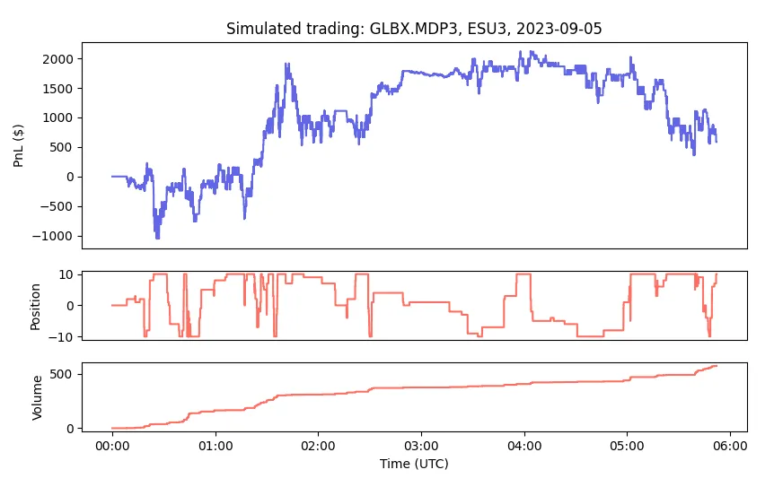
 A high-frequency liquidity-taking strategy
We'll introduce some terminology for this tutorial:
- A feature is any kind of basic independent variable that we think has some predictive value. This follows machine learning nomenclature; others may refer to this as a predictor or regressor in a statistical or econometric setting.
- A trading rule is a hardcoded trading decision. An example of a trading rule is "If there's only 1 order left at the best offer, lift the offer; if there is only 1 order left at the best bid, hit the bid". A trading rule may be a hardcoded trading decision taken when a feature value exceeds a certain threshold.
- A strategy that is based on trading rules is a rule-based strategy.
- A liquidity-taking strategy takes liquidity by crossing the spread with aggressive or marketable orders.
- A high-frequency strategy is characterized by a large number of trades.
Book skew and trading rule
The simplest type of book feature is called the book skew, which is the imbalance between resting bid depth (vb) and resting ask depth (va) at the top of the book. We can formulate this as some sort of difference between vb and va. It's convenient to scale these by their order of magnitude, so we take their log differences instead.
skew=log(vb)−log(va)=logvavbNotice that we picked this ordering simply because it's useful to formulate features such that positive values imply that we expect prices to go up; this makes it easier to debug your strategy. Intuitively, we expect higher bid depth to imply higher buy demand and hence higher prices.
We can introduce a trading rule that buys when this feature exceeds some alpha
threshold k, and sells when it goes below some threshold -k.
Minimum order quantity
While there's some practical advantage to trading larger clips for a liquidity-taking strategy, we'll start with a constant trade size equal to the minimum order quantity so that we minimize slippage and market impact considerations.
The minimum order quantity depends on the trading platform or market that you're on. For this toy strategy, we'll use E-mini S&P 500 (ES) futures as an example and trade in clips of 1 contract.
skew>k→Buy 1 lotskew<−k→Sell 1 lotCommissions
This strategy will be very sensitive to commissions due to its volume, so we'll include commissions on the estimated PnL. These commissions can be found here.
Position and risk limits
This strategy is convenient because you don't have to worry about complex order and position state management. You just let it build up whatever maximum position you want. Because we expect buys and sells to be symmetrically distributed in the long run, you will eventually get out of position. However, you might not have enough margin to build up arbitrarily large positions, so for proof of concept, we'll specify a maximum position of 10 contracts.
skew>k and pos<10 lots→Buy 1 lotskew<−k and pos>−10 lots→Sell 1 lotImplementation
These are the parameters we have so far:
Info
import math
import json
import sys
from dataclasses import dataclass, field
from decimal import Decimal

import pandas as pd
import databento as db

API_KEY = "YOUR_API_KEY"


class Config:

    # Alpha threshold to buy/sell, k
    ALPHA_THRESHOLD: int = 1.7

    # Symbol
    DATASET = "GLBX.MDP3"
    SYMBOL = "ESU3"
    POINT_VALUE = 50    # $50 per index point

    # Fees
    VENUE_FEES_PER_SIDE: Decimal = Decimal("0.39")
    CLEARING_FEES_PER_SIDE: Decimal = Decimal("0.05")
    FEES_PER_SIDE: Decimal = VENUE_FEES_PER_SIDE + CLEARING_FEES_PER_SIDE

    # Position limit
    POSITION_MAX: int = 10
Since we're only simulating liquidity-taking at minimum size, our MBP-1 schema is sufficient. You can learn more about our MBP-1 schema here.
To keep this example simple, we'll assume zero round-trip latency for any orders placed. This enables us to implement a simple, online calculation of PnL for our real-time trading simulation.
@dataclass(slots=True)
class Strategy:

    # Dataset
    dataset: str

    # Instrument to trade
    symbol: str

    # Current position, in contract units
    position: int = 0
    # Number of long contract sides traded
    buy_qty: int = 0
    # Number of short contract sides traded
    sell_qty: int = 0

    ## Total realized buy price
    real_total_buy_px: Decimal = 0
    ## Total realized sell price
    real_total_sell_px: Decimal = 0

    # Total buy price to liquidate current position
    theo_total_buy_px: Decimal = 0
    # Total sell price to liquidate current position
    theo_total_sell_px: Decimal = 0

    # Total fees paid
    fees: Decimal = 0

    # List to track results
    results: list = field(default_factory=list)

    def run(self) -> None:
        client = db.Live()
        client.subscribe(
            dataset=self.dataset,
            schema="mbp-1",
            stype_in="raw_symbol",
            symbols=[self.symbol],
            # start="2023-08-08T12:00",    # Burn-in start time
        )
        for record in client:
            if not isinstance(record, db.MBP1Msg):
                continue
            self.update(record)

    def update(self, record: db.MBP1Msg) -> None:
        ask_size = record.levels[0].ask_sz
        bid_size = record.levels[0].bid_sz
        ask_price = record.levels[0].ask_px / Decimal("1e9")
        bid_price = record.levels[0].bid_px / Decimal("1e9")

        skew = math.log10(bid_size) - math.log10(ask_size)
        mid_price = (ask_price + bid_price) / 2

        # Buy/sell based when skew signal is large
        if skew > Config.ALPHA_THRESHOLD and self.position < Config.POSITION_MAX:
            self.position += 1
            self.buy_qty += 1
            self.real_total_buy_px += ask_price
            self.fees += Config.FEES_PER_SIDE
        elif skew < -Config.ALPHA_THRESHOLD and self.position > -Config.POSITION_MAX:
            self.position -= 1
            self.sell_qty += 1
            self.real_total_sell_px += bid_price
            self.fees += Config.FEES_PER_SIDE

        # Update prices
        # Fill prices are based on BBO with assumed zero latency
        # In practice, should be worse because of alpha decay
        if self.position == 0:
            self.theo_total_buy_px = 0
            self.theo_total_sell_px = 0
        elif self.position > 0:
            self.theo_total_sell_px = bid_price * abs(self.position)
        elif self.position < 0:
            self.theo_total_buy_px = ask_price * abs(self.position)

        # Compute PnL
        theo_pnl = (
            Config.POINT_VALUE
            * (
                self.real_total_sell_px
                + self.theo_total_sell_px
                - self.real_total_buy_px
                - self.theo_total_buy_px
            )
            - self.fees
        )

        result = {
            "ts_strategy": str(pd.Timestamp(record.ts_recv, tz="UTC")),
            "bid": f"{bid_price:0.2f}",
            "ask": f"{ask_price:0.2f}",
            "skew" : f"{skew:0.3f}",
            "position": self.position,
            "trade_ct": self.buy_qty + self.sell_qty,
            "fees": f"{self.fees:0.2f}",
            "pnl": f"{theo_pnl:0.2f}",
        }

        print(json.dumps(result, indent=4))

        self.results.append(result)


if __name__ == "__main__":
    strategy = Strategy(dataset=Config.DATASET, symbol=Config.SYMBOL)
    while True:
        try:
            strategy.run()
        except KeyboardInterrupt:
            df = pd.DataFrame(strategy.results)
            df.to_csv("strategy_log.csv", index=False)
            sys.exit()
Results
Further improvements
This implementation uses our simple synchronous client. For production applications, we recommend using our asynchronous client or callback model.
A problem encountered with the book skew is that extreme values may be influenced by spoofing. One possibility is to modify the trading rule and introduce an upper limit as follows:
skew>k and abs(skew)<L and pos<10 lots→Buy 1 lotskew<−k and abs(skew)<L and pos>−10 lots→Sell 1 lotFinally, recall that we assumed zero delay in order placement and fill. It's also important to incorporate a delay when extending this example.