Python example: How to get options with the underlying asset

This example builds off the Join schemas on instrument ID example.

Overview

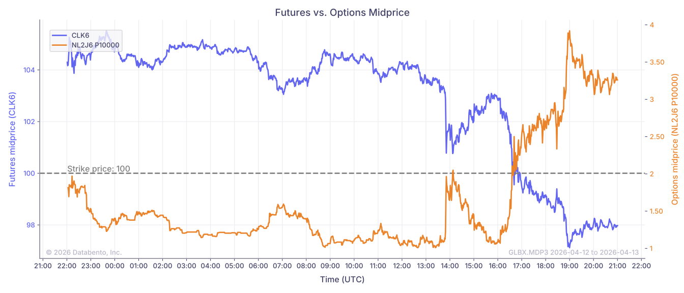
In this example, we'll use the Historical client to data for futures and options. First, we'll request trades schema data for all options on the volume-based continuous contract and join them with the most recent quote from the MBP-1 schema for the underlying future. We'll also request BBO-1m schema data for the underlying future and a single option and plot the midprice for a full session.

Example

import databento as db
import matplotlib.dates as mdates
import matplotlib.pyplot as plt
import pandas as pd

def get_bbo_data(
    dataset: str,
    instrument_id: int,
    start: str,
    end: str,
) -> pd.DataFrame:
    mbp_df = client.timeseries.get_range(
        dataset=dataset,
        schema="bbo-1m",
        symbols=instrument_id,
        stype_in="instrument_id",
        start=start,
        end=end,
    ).to_df(map_symbols=False)
    return mbp_df[["instrument_id", "bid_px_00", "ask_px_00"]]

def plot_option_with_underlying(
    opt_df: pd.DataFrame,
    fut_df: pd.DataFrame,
) -> None:
    opt_df["mid_price"] = (opt_df["bid_px_00"] + opt_df["ask_px_00"]) / 2
    fut_df["mid_price"] = (fut_df["bid_px_00"] + fut_df["ask_px_00"]) / 2

    full_index = pd.date_range(
        start=start,
        end=end,
        freq="1min",
        tz="UTC",
        inclusive="right",
    )
    opt_df = opt_df.reindex(full_index).ffill().astype(opt_df.dtypes)
    fut_df = fut_df.reindex(full_index).ffill().astype(fut_df.dtypes)

    opt_symbol = opt_df["raw_symbol"].iloc[0]
    fut_symbol = opt_df["underlying"].iloc[0]

    fig, ax1 = plt.subplots(figsize=(14, 6))

    ax1.plot(fut_df.index, fut_df["mid_price"], color="C0", label=fut_symbol)
    ax1.set_ylabel(f"Futures midprice ({fut_symbol})", color="C0")
    ax1.tick_params(axis="y", labelcolor="C0")

    strike = opt_df["strike_price"].iloc[0]
    ax1.axhline(y=strike, color="gray", linestyle="--")
    ax1.text(
        x=fut_df.index[0],
        y=strike,
        s=f"Strike price: {strike:.0f}",
        color="gray",
        va="bottom",
        ha="left",
    )

    ax2 = ax1.twinx()
    ax2.plot(opt_df.index, opt_df["mid_price"], color="C1", label=opt_symbol)
    ax2.set_ylabel(f"Options midprice ({opt_symbol})", color="C1")
    ax2.tick_params(axis="y", labelcolor="C1")

    ax1.xaxis.set_major_formatter(mdates.DateFormatter("%H:%M"))
    ax1.xaxis.set_major_locator(mdates.HourLocator(interval=1))

    ax1.set_title("Futures vs. Options Midprice")
    ax1.set_xlabel("Time (UTC)")

    lines1, labels1 = ax1.get_legend_handles_labels()
    lines2, labels2 = ax2.get_legend_handles_labels()
    ax1.legend(lines1 + lines2, labels1 + labels2, loc="upper left")

    ax1.grid(True)
    ax2.grid(False)

    fig.tight_layout()
    plt.show()

# Create a historical client
client = db.Historical("$YOUR_API_KEY")

# Set parameters
dataset = "GLBX.MDP3"
symbol = "CL.v.0"
start = "2026-04-12T22:00:00"
end = "2026-04-13T21:00:00"

# Get symbol mapping for the continuous contract
symbol_map = client.symbology.resolve(
    dataset=dataset,
    symbols=symbol,
    stype_in="continuous",
    stype_out="instrument_id",
    start_date="2026-04-12",
)
# Get instrument ID for the resolved futures contract
fut_id = int(symbol_map["result"][symbol][0]["s"])

# Get all option definitions
def_df = client.timeseries.get_range(
    dataset=dataset,
    symbols="ALL_SYMBOLS",
    schema="definition",
    start="2026-04-12",
).to_df()

# Filter for options with the continuous contract as an underlying
opt_def_df = def_df[
    (def_df["user_defined_instrument"] == db.UserDefinedInstrument.NO) &
    (def_df["instrument_class"].isin((db.InstrumentClass.CALL, db.InstrumentClass.PUT))) &
    (def_df["underlying_id"] == fut_id)
]
opt_def_df = opt_def_df[["ts_event", "expiration", "raw_symbol", "instrument_id", "asset", "strike_price", "underlying", "underlying_id", "instrument_class"]]

# Get trades data for the filtered options
opt_trades_df = client.timeseries.get_range(
    dataset=dataset,
    schema="trades",
    symbols=[f"{x}.OPT" for x in opt_def_df["asset"].unique()],
    stype_in="parent",
    start=start,
    end=end,
).to_df().rename(columns={"size": "trade_size", "price": "trade_price", "side": "trade_side"})

# Join options with their definitions
opt_df = opt_trades_df.reset_index().merge(
    opt_def_df.reset_index(),
    on="instrument_id",
    how="inner",
    suffixes=("", "_def"),
).set_index("ts_recv").sort_index()

fut_mbp_df = client.timeseries.get_range(
    dataset=dataset,
    schema="mbp-1",
    symbols=fut_id,
    stype_in="instrument_id",
    start=start,
    end=end,
).to_df()
fut_mbp_df = fut_mbp_df.rename(
    columns={
        "bid_px_00": "underlying_bid",
        "ask_px_00": "underlying_ask",
    },
)[["underlying_bid", "underlying_ask"]]

# Join most recent underlying bid/ask with options trades
df = pd.merge_asof(
    opt_df,
    fut_mbp_df,
    left_index=True,
    right_index=True,
    direction="backward",
)

print(df[["ts_event", "instrument_id", "raw_symbol", "trade_price", "trade_size", "trade_side", "strike_price", "instrument_class", "expiration", "underlying_bid", "underlying_ask"]])

# 42963414 is the `instrument_id` for NL2J6 P10000
opt_id = 42963414
opt_bbo_df = get_bbo_data(dataset, opt_id, start, end)
opt_bbo_df = opt_bbo_df.reset_index().merge(opt_def_df, on="instrument_id", how="left").set_index("ts_recv")

fut_bbo_df = get_bbo_data(dataset, fut_id, start, end)

plot_option_with_underlying(opt_bbo_df, fut_bbo_df)

Result

We can see all trades for options that have the volume-based continuous contract as an underlying.

                                                               ts_event  instrument_id    raw_symbol  trade_price  trade_size  ... strike_price  instrument_class                expiration underlying_bid  underlying_ask
ts_recv                                                                                                                        ...
2026-04-12 22:00:00.356333832+00:00           2026-04-12 22:00:00+00:00       42157669    LOK6 C9900         6.01           1  ...        99.00                 C 2026-04-16 18:30:00+00:00            NaN             NaN
2026-04-12 22:00:00.356370138+00:00           2026-04-12 22:00:00+00:00       42180553    LOK6 P8200         0.39           1  ...        82.00                 P 2026-04-16 18:30:00+00:00            NaN             NaN
2026-04-12 22:00:00.357402871+00:00           2026-04-12 22:00:00+00:00       42511805  ML2J6 C10000         2.40           2  ...       100.00                 C 2026-04-13 18:30:00+00:00            NaN             NaN
2026-04-12 22:00:00.357526014+00:00           2026-04-12 22:00:00+00:00       42639465   ML2J6 P9100         0.74           1  ...        91.00                 P 2026-04-13 18:30:00+00:00            NaN             NaN
2026-04-12 22:00:00.357609934+00:00           2026-04-12 22:00:00+00:00       42963412   NL2J6 P9600         0.99           1  ...        96.00                 P 2026-04-14 18:30:00+00:00            NaN             NaN
...                                                                 ...            ...           ...          ...         ...  ...          ...               ...                       ...            ...             ...
2026-04-13 20:57:18.223377118+00:00 2026-04-13 20:57:18.222967937+00:00       42308894    LOK6 P8500         0.27           1  ...        85.00                 P 2026-04-16 18:30:00+00:00          97.96           97.98
2026-04-13 20:57:18.223891862+00:00 2026-04-13 20:57:18.223423419+00:00       42308894    LOK6 P8500         0.27           1  ...        85.00                 P 2026-04-16 18:30:00+00:00          97.96           97.98
2026-04-13 20:57:19.267462126+00:00 2026-04-13 20:57:19.267057293+00:00       42631933   WL3J6 C9775         3.03           1  ...        97.75                 C 2026-04-15 18:30:00+00:00          97.97           97.99
2026-04-13 20:58:04.991697756+00:00 2026-04-13 20:58:04.983728493+00:00       42958534  NL2J6 C10100         0.91           1  ...       101.00                 C 2026-04-14 18:30:00+00:00          97.94           97.96
2026-04-13 20:58:38.292464827+00:00 2026-04-13 20:58:38.292053561+00:00         379004    LOK6 P7000         0.02           1  ...        70.00                 P 2026-04-16 18:30:00+00:00          97.97           97.99

[17262 rows x 11 columns]

Now we'll plot the midprice of the underlying future and a single option for the duration of a full session. In this example, the option NL2J6 P10000 expires on 2026-04-14.

Join options with underlying prices

Overview

Example

Result