Build prediction models with machine learning
Overview
In this example we will use the Historical client to build high-frequency trading signals and use them to train a machine learning model.
MBP-10 schema
We'll demonstrate this example using the MBP-10 schema. The MBP-10 schema contains the top ten levels of aggregated book depth. This updates on every order book event.
Dependencies
This example will use the scikit-learn package for creating a machine learning model. The matplotlib package will be used for charting.
These dependencies can be installed with the following:
1
$ pip install scikit-learn matplotlib
Example
1
2
3
4
5
6
7
8
9
10
11
12
13
14
15
16
17
18
19
20
21
22
23
24
25
26
27
28
29
30
31
32
33
34
35
36
37
38
39
40
41
42
43
44
45
46
47
48
49
50
51
52
53
54
55
56
57
58
59
60
61
62
63
64
65
66
67
68
69
70
71
72
73
74
75
76
77
78
79
80
81
82
83
84
85
86
87
88
89
90
91
import databento as db
import matplotlib.pyplot as plt
import numpy as np
import pandas as pd
from sklearn.linear_model import LinearRegression

# Create a historical client
client = db.Historical(key="$YOUR_API_KEY")

# Set parameters
dataset = "GLBX.MDP3"
product = "ES"
start = "2023-12-06T14:30:00"
end = "2023-12-06T20:33:00"

# Request MBP-10 for the front-month ES contract and convert to DataFrame
df = client.timeseries.get_range(
    dataset="GLBX.MDP3",
    schema="mbp-10",
    symbols=f"{product}.v.0",
    stype_in="continuous",
    start=start,
    end=end,
).to_df()

# Filter out trades only
df = df[df["action"] == db.Action.TRADE]

# Calculate midprice returns with a forward markout of 500 trades
df["mid"] = (df["bid_px_00"] + df["ask_px_00"]) / 2
df["ret_500t"] = df["mid"].shift(-500) - df["mid"]
df = df.dropna()

# Calculate depth imbalance on top level ('skew')
df["skew"] = np.log(df.bid_sz_00) - np.log(df.ask_sz_00)

# Calculate order imbalance on top ten levels ('imbalance')
bid_count = df[list(df.filter(regex="bid_ct_0[0-9]"))].sum(axis=1)
ask_count = df[list(df.filter(regex="ask_ct_0[0-9]"))].sum(axis=1)
df["imbalance"] = np.log(bid_count) - np.log(ask_count)

# Split in-sample and out-of-sample
split = int(0.66 * len(df))
split -= split % 100
df_in = df.iloc[:split]
df_out = df.iloc[split:]

# Evaluate signal correlation
corr = df_in[["skew", "imbalance", "ret_500t"]].corr()
print(corr.where(np.triu(np.ones(corr.shape)).astype(bool)))

reg = LinearRegression(fit_intercept=False, positive=True)

# Create a model using skew only
reg.fit(df_in[["skew"]], df_in["ret_500t"])
pred_skew = reg.predict(df_out[["skew"]])

# Create a model using imbalance only
reg.fit(df_in[["imbalance"]], df_in["ret_500t"])
pred_imbalance = reg.predict(df_out[["imbalance"]])

# Create a model using both skew and imbalance
reg.fit(df_in[["skew", "imbalance"]], df_in["ret_500t"])
pred_combined = reg.predict(df_out[["skew", "imbalance"]])


# Define a function to calculate profit and loss
def get_cumulative_markout_pnl(pred):
    df_pnl = pd.DataFrame({"pred": pred, "ret_500t": df_out["ret_500t"].values})
    df_pnl.loc[df_pnl["pred"] < 0, "ret_500t"] *= -1
    df_pnl = df_pnl.sort_values(by="pred")
    return df_pnl["ret_500t"].cumsum().values


# Collect results into a DataFrame
results = pd.DataFrame(
    {
        "skew": get_cumulative_markout_pnl(pred_skew),
        "imbalance": get_cumulative_markout_pnl(pred_imbalance),
        "combined": get_cumulative_markout_pnl(pred_combined),
    },
    index=np.linspace(0, 100, num=len(df_out)),
)

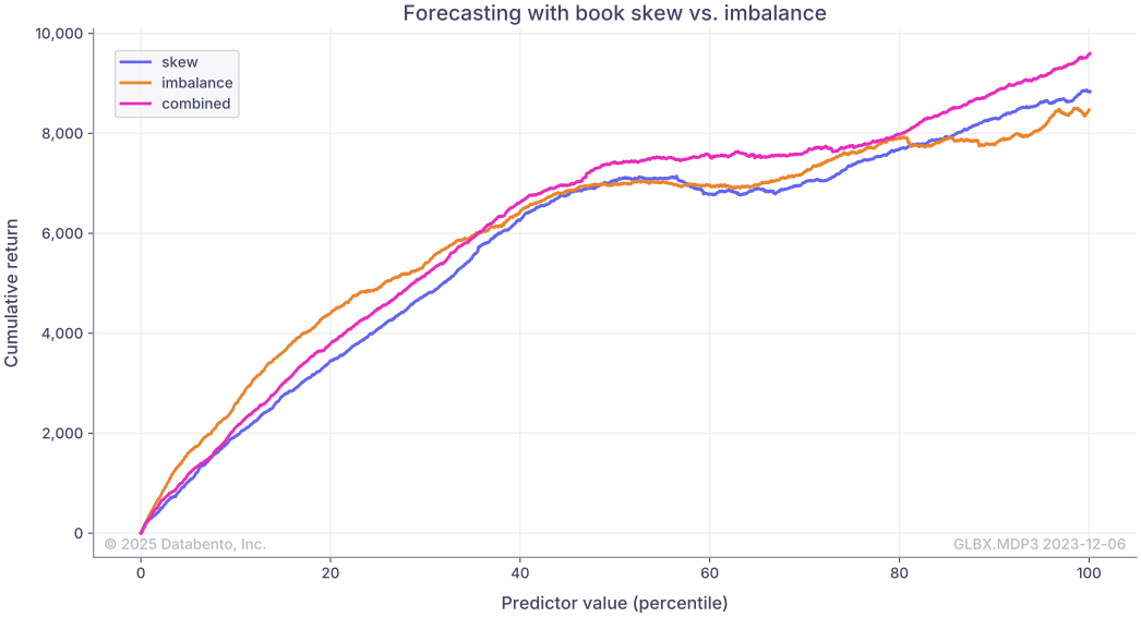
# Plot the results
results.plot(
    title="Forecasting with book skew vs. imbalance",
    xlabel="Predictor value (percentile)",
    ylabel="Cumulative return",
).legend()
plt.show()
Result
1
2
3
4
           skew  imbalance  ret_500t
skew        1.0    0.47513  0.109004
imbalance   NaN    1.00000  0.064666
ret_500t    NaN        NaN  1.000000