Analyze auction imbalance dynamics
The closing auction for US Equities is one of the most important events of the trading day. With nearly 10% of average daily volume transacting on the close, the dynamics around price discovery are critical, as these closing prices are used in various use cases, such as benchmark pricing for index funds. While different exchanges share many common behaviors during the closing auction, there are some microstructure differences, such as accepted order types, that can affect the price discovery mechanism.
Overview
We'll use the historical client to request data for the closing auction. The imbalance schema provides auction imbalance data such as reference price, paired quantity, and auction status. We'll also use the OHLCV-1m schema to look at the price and volume transacting on the limit order book.
We'll compare the closing auction process for SPY on NYSE Arca and QQQ on Nasdaq. Due to differences in the data disseminated by the exchange, we'll use different fields for Nasdaq and NYSE.
For both venues, the ref_price field represents the price at which imbalance shares are being calculated. This price is generally within the current BBO on the limit order book.
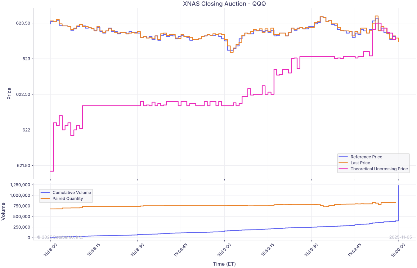
For Nasdaq, we'll look at the cont_book_clr_price field, which represents the price at which auction and continuous orders would transact.
For NYSE Arca, we'll look at the ind_match_price field instead. This field represents the price at which the highest number of shares would trade, subject to auction collars.
Example
1
2
3
4
5
6
7
8
9
10
11
12
13
14
15
16
17
18
19
20
21
22
23
24
25
26
27
28
29
30
31
32
33
34
35
36
37
38
39
40
41
42
43
44
45
46
47
48
49
50
51
52
53
54
55
56
57
58
59
60
61
62
63
64
65
66
67
68
69
70
71
72
73
74
75
76
77
78
79
80
81
82
83
84
85
86
87
88
89
90
91
92
93
94
95
96
97
98
99
100
101
102
103
104
105
106
107
108
109
110
111
112
113
114
115
116
117
118
119
120
121
122
123
124
125
126
127
128
129
130
131
132
133
134
135
136
137
138
139
140
141
142
143
144
145
146
147
148
149
150
151
152
153
154
155
156
157
158
159
160
161
162
163
164
165
import datetime as dt
from zoneinfo import ZoneInfo
import databento as db
import pandas as pd
from matplotlib import dates as mdates
from matplotlib import pyplot as plt

def get_imbalance_df(
    client: db.Historical,
    dataset: str,
    symbol: str,
    start: dt.datetime,
    end: dt.datetime,
) -> pd.DataFrame:
    """Get imbalance schema data"""
    imbalance_df = client.timeseries.get_range(
        dataset=dataset,
        symbols=symbol,
        schema="imbalance",
        start=start,
        end=end,
    ).to_df(tz=start.tzinfo)

    return imbalance_df


def get_ohlcv_df(
    client: db.Historical,
    dataset: str,
    symbol: str,
    start: dt.datetime,
    end: dt.datetime,
) -> pd.DataFrame:
    """Get OHLCV schema data"""
    ohlcv_df = client.timeseries.get_range(
        dataset=dataset,
        symbols=symbol,
        schema="ohlcv-1s",
        start=start,
        end=end,
    ).to_df(tz=start.tzinfo)

    return ohlcv_df


def plot_closing_auction(
    venue: str,
    symbol: str,
    imbalance_df: pd.DataFrame,
    ohlcv_df: pd.DataFrame,
    start_time: dt.time,
    end_time: dt.time,
) -> None:
    imbalance_df = imbalance_df.between_time(start_time, end_time)

    ohlcv_df = ohlcv_df.between_time(start_time, end_time)
    ohlcv_df["cumulative_volume"] = ohlcv_df["volume"].cumsum()

    # Create the subplots
    _, (ax1, ax2) = plt.subplots(
        2,
        1,
        figsize=(14, 9),
        sharex=True,
        gridspec_kw={"height_ratios": [3, 1]},
    )

    # First subplot will display prices
    ax1.plot(
        imbalance_df.index,
        imbalance_df["ref_price"],
        label="Reference Price",
        drawstyle="steps-pre",
    )

    ax1.plot(
        ohlcv_df.index,
        ohlcv_df["close"],
        label="Last Price",
        drawstyle="steps-post",
    )

    ax1.plot(
        imbalance_df.index,
        imbalance_df["uncrossing_price"],
        label="Theoretical Uncrossing Price",
        drawstyle="steps-post",
    )

    ax1.set_ylabel("Price")
    ax1.grid(True)
    ax1.legend(loc="best")
    ax1.set_title(f"{venue} Closing Auction - {symbol}")

    # Second subplot will display traded volume and auction paired quantity
    ax2.plot(
        ohlcv_df.index,
        ohlcv_df["cumulative_volume"],
        label="Cumulative Volume",
        drawstyle="steps-post",
    )

    ax2.plot(
        imbalance_df.index,
        imbalance_df["paired_qty"],
        label="Paired Quantity",
        drawstyle="steps-post",
    )

    ax2.set_xlabel("Time (ET)")
    ax2.set_ylabel("Volume")
    ax2.grid(True)
    ax2.legend(loc="best")
    ax2.xaxis.set_major_formatter(mdates.DateFormatter("%H:%M:%S", tz=start_time.tzinfo))
    plt.xticks(rotation=45)

    plt.show()


# Set parameters
tz = ZoneInfo("America/New_York")
start = dt.datetime(2025, 11, 5, 15, 58, 0, tzinfo=tz)
end = dt.datetime(2025, 11, 5, 16, 0, 1, tzinfo=tz)

client = db.Historical("$YOUR_API_KEY")

# First, we'll look at SPY data on NYSE Arca (ARCX.PILLAR)
arcx_symbol = "SPY"
arcx_dataset = "ARCX.PILLAR"

arcx_ohlcv_df = get_ohlcv_df(client, arcx_dataset, arcx_symbol, start, end)
arcx_imbalance_df = get_imbalance_df(client, arcx_dataset, arcx_symbol, start, end)
arcx_imbalance_df = arcx_imbalance_df.rename(columns={"ind_match_price": "uncrossing_price"})
arcx_imbalance_df = arcx_imbalance_df[["ref_price", "uncrossing_price", "paired_qty", "symbol"]]

print(arcx_imbalance_df)

plot_closing_auction(
    "ARCX",
    arcx_symbol,
    arcx_imbalance_df,
    arcx_ohlcv_df,
    dt.time(15, 58, 0, tzinfo=tz),
    dt.time(16, 0, 0, tzinfo=tz),
)

# Next, we'll look at QQQ data on Nasdaq (XNAS.ITCH)
xnas_symbol = "QQQ"
xnas_dataset = "XNAS.ITCH"

xnas_ohlcv_df = get_ohlcv_df(client, xnas_dataset, xnas_symbol, start, end)
xnas_imbalance_df = get_imbalance_df(client, xnas_dataset, xnas_symbol, start, end)
xnas_imbalance_df = xnas_imbalance_df.rename(columns={"cont_book_clr_price": "uncrossing_price"})
xnas_imbalance_df = xnas_imbalance_df[["ref_price", "uncrossing_price", "paired_qty", "symbol"]]

print(xnas_imbalance_df)

plot_closing_auction(
    "XNAS",
    xnas_symbol,
    xnas_imbalance_df,
    xnas_ohlcv_df,
    dt.time(15, 58, 0, tzinfo=tz),
    dt.time(16, 0, 0, tzinfo=tz),
)
Results
First, we'll take a look at the closing auction for SPY on NYSE Arca.
See the NYSE Arca auction documentation for more information.
1
2
3
4
5
6
7
8
9
10
11
12
13
                                     ref_price  uncrossing_price  paired_qty symbol
ts_recv
2025-11-05 15:58:00.061423353-05:00    677.715            684.49      951885    SPY
2025-11-05 15:58:01.055768239-05:00    677.760            676.22     1193528    SPY
2025-11-05 15:58:02.054678442-05:00    677.760            676.50     1194940    SPY
2025-11-05 15:58:03.056152198-05:00    677.760            676.50     1195106    SPY
2025-11-05 15:58:04.054268311-05:00    677.720            676.18     1200714    SPY
...                                        ...               ...         ...    ...
2025-11-05 15:59:55.052843213-05:00    677.670            677.81     1401805    SPY
2025-11-05 15:59:56.050469422-05:00    677.600            677.76     1402565    SPY
2025-11-05 15:59:57.051653917-05:00    677.590            677.72     1402565    SPY
2025-11-05 15:59:58.052726733-05:00    677.530            677.68     1403065    SPY
2025-11-05 15:59:59.050924091-05:00    677.470            677.60     1403218    SPY
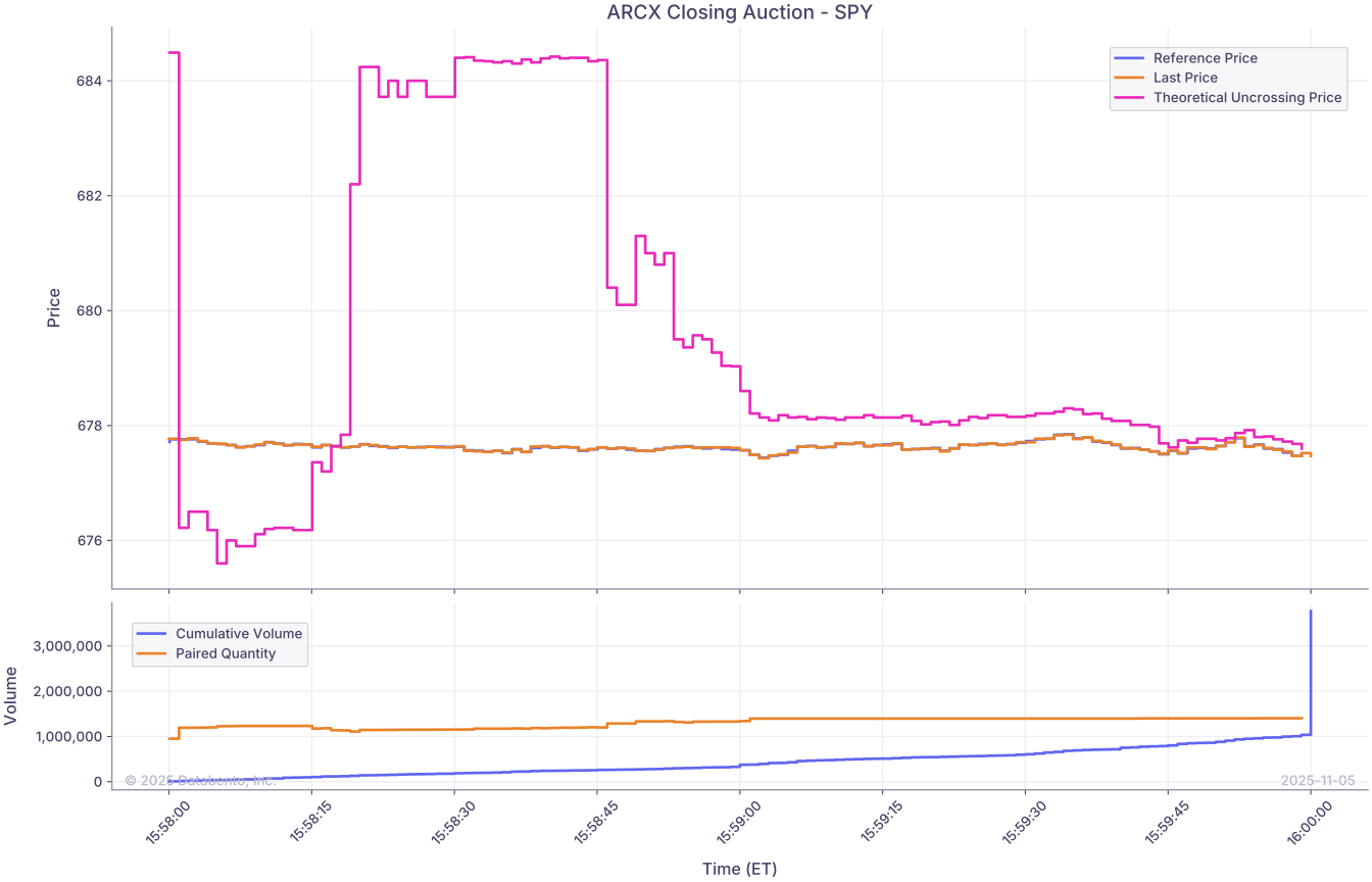
Next, we'll look at the closing auction for QQQ on Nasdaq. You'll notice that in both examples, these theoretical uncrossing prices will converge towards the last traded price as we approach the close.
See the Nasdaq Closing Cross documentation for more information.
1
2
3
4
5
6
7
8
9
10
11
12
13
                                     ref_price  uncrossing_price  paired_qty symbol
ts_recv
2025-11-05 15:58:00.060035531-05:00     623.49            621.42      677169    QQQ
2025-11-05 15:58:01.019052477-05:00     623.52            622.10      677696    QQQ
2025-11-05 15:58:02.055023604-05:00     623.52            622.06      678796    QQQ
2025-11-05 15:58:03.010276615-05:00     623.54            622.20      678836    QQQ
2025-11-05 15:58:04.040411490-05:00     623.47            622.00      699336    QQQ
...                                        ...               ...         ...    ...
2025-11-05 15:59:55.008542818-05:00     623.43            623.43      827157    QQQ
2025-11-05 15:59:56.099171134-05:00     623.37            623.37      826774    QQQ
2025-11-05 15:59:57.059011900-05:00     623.36            623.36      826774    QQQ
2025-11-05 15:59:58.025345576-05:00     623.27            623.27      826393    QQQ
2025-11-05 15:59:59.032786745-05:00     623.31            623.31      826393    QQQ