Daily statistics for equity options
Overview
In this example, we'll use the Historical client to calculate volume and open interest statistics for an equity options chain.
First, we'll use the definition schema, which contains instrument definitions and properties, to get information such as expiration, strike_price, and instrument_class. Next, we'll use the OHLCV-1d schema to get the total volume for each option. Finally, we'll use the statistics schema to request open interest statistics. OPRA publishes start-of-day open interest statistics before the regular trading hours (RTH) open at 9:30 ET.
Example
1
2
3
4
5
6
7
8
9
10
11
12
13
14
15
16
17
18
19
20
21
22
23
24
25
26
27
28
29
30
31
32
33
34
35
36
37
38
39
40
41
42
43
44
45
46
47
48
49
50
51
52
53
54
55
56
57
58
59
60
61
62
63
64
65
66
67
68
69
70
71
72
73
74
75
76
77
78
79
80
81
82
83
84
85
86
87
88
89
90
91
92
93
94
95
96
97
98
99
100
101
102
103
104
105
106
107
108
109
110
111
112
113
114
115
116
117
118
119
120
121
122
123
124
125
126
127
128
129
130
131
132
133
134
135
136
137
import datetime as dt
from zoneinfo import ZoneInfo
import databento as db
import matplotlib.pyplot as plt
import pandas as pd
from matplotlib.patches import Patch
from matplotlib.ticker import MaxNLocator

def get_volume_data(
    client: db.Historical,
    dataset: str,
    symbol: str,
    date: dt.date,
) -> pd.DataFrame:
    """Get volume data for all options for a given symbol."""
    volume_df = client.timeseries.get_range(
        dataset=dataset,
        symbols=f"{symbol}.OPT",
        schema="ohlcv-1d",
        stype_in="parent",
        start=date,
    ).to_df()

    return volume_df.groupby("symbol")["volume"].sum().reset_index()


def get_oi_data(
    client: db.Historical,
    dataset: str,
    symbol: str,
    date: dt.date,
) -> pd.DataFrame:
    """Get open interest data for all options for a given symbol."""
    # Start-of-day open interest is published before the RTH open at 9:30 ET
    end_time = dt.time(9, 30, 0, tzinfo=ZoneInfo("America/New_York"))
    stats_df = client.timeseries.get_range(
        dataset=dataset,
        symbols=f"{symbol}.OPT",
        schema="statistics",
        stype_in="parent",
        start=date,
        end=dt.datetime.combine(date, end_time),
    ).to_df()

    stats_df = stats_df[stats_df["stat_type"] == db.StatType.OPEN_INTEREST]
    stats_df = stats_df.drop_duplicates("symbol", keep="last")
    stats_df["open_interest"] = stats_df[stats_df["stat_type"] == db.StatType.OPEN_INTEREST][
        "quantity"
    ]

    return stats_df[["open_interest", "symbol"]]


def get_definition_data(
    client: db.Historical,
    dataset: str,
    symbol: str,
    date: dt.date,
) -> pd.DataFrame:
    """Get definition data for all options for a given symbol."""
    def_df = client.timeseries.get_range(
        dataset=dataset,
        symbols=f"{symbol}.OPT",
        schema="definition",
        stype_in="parent",
        start=date,
    ).to_df()

    def_df["days_to_expiration"] = (def_df["expiration"] - def_df.index.normalize()).dt.days
    def_df["expiration"] = def_df["expiration"].dt.normalize().dt.date

    return def_df[
        ["symbol", "strike_price", "instrument_class", "expiration", "days_to_expiration"]
    ]


def plot_oi_by_strike(
    df: pd.DataFrame,
    expiration_date: dt.date,
) -> None:
    df = df[df["expiration"] == expiration_date]
    trade_date = df["trade_date"].iloc[0]
    days_to_expiration = df["days_to_expiration"].iloc[0]

    df_strikes = df.groupby(["strike_price", "instrument_class"])["open_interest"].sum().unstack()

    # Plot bar chart
    _, ax = plt.subplots(figsize=(14, 6))
    df_strikes.plot(
        ax=ax,
        kind="bar",
        xlabel="Strike price",
        ylabel="Open interest",
    )

    # Adjust X ticks and labels
    ax.xaxis.set_major_locator(MaxNLocator(15))
    ax.set_xticklabels(ax.get_xticklabels(), rotation=45, ha="right")

    # Set title and legend
    ax.set_title(f"{symbol} open interest \n {trade_date} ({days_to_expiration} DTE)")
    ax.legend(handles=[Patch(facecolor="C0", label="Call"), Patch(facecolor="C1", label="Put")])

    plt.tight_layout()
    plt.show()


# Set parameters
dataset = "OPRA.PILLAR"
symbol = "NVDA"
start = dt.date(2025, 8, 19)

# Create a historical client
client = db.Historical("$YOUR_API_KEY")

# Get strike price, expiration, and instrument class in the definition schema
def_df = get_definition_data(client, dataset, symbol, start)

# Volume from the OHLCV-1d schema
volume_df = get_volume_data(client, dataset, symbol, start)

# Start-of-day open interest is published in the morning in the statistics schema
stats_df = get_oi_data(client, dataset, symbol, start)

# Merge different schemas together
df = def_df.merge(volume_df, on="symbol", how="left")
df = df.merge(stats_df, on="symbol", how="left")

df["trade_date"] = start
df["volume"] = df["volume"].fillna(0).astype(int)
df["open_interest"] = df["open_interest"].fillna(0).astype(int)

# Print out top 10 contracts by open interest
print(df.nlargest(10, "open_interest").to_string(index=False))

# Plot open interest by expiration date
plot_oi_by_strike(df, dt.date(2025, 8, 22))
Result
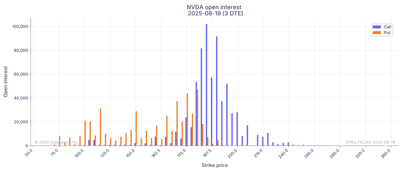
You could use the resulting data to filter for the contracts with the highest open interest. Additionally, you could plot the open interest distribution for a given expiration.
1
2
3
4
5
6
7
8
9
10
11
               symbol  strike_price instrument_class expiration  days_to_expiration  volume  open_interest trade_date
NVDA  250919C00160000         160.0                C 2025-09-19                  31   52206         173864 2025-08-19
NVDA  260618P00075000          75.0                P 2026-06-18                 303       1         109796 2025-08-19
NVDA  250919C00170000         170.0                C 2025-09-19                  31    4636         106760 2025-08-19
NVDA  250822C00185000         185.0                C 2025-08-22                   3  158486         102111 2025-08-19
NVDA  250919C00185000         185.0                C 2025-09-19                  31   61860         101843 2025-08-19
NVDA  250919C00190000         190.0                C 2025-09-19                  31   59766          92379 2025-08-19
NVDA  250822C00190000         190.0                C 2025-08-22                   3   46489          91666 2025-08-19
NVDA  250919C00165000         165.0                C 2025-09-19                  31     759          90851 2025-08-19
NVDA  250919C00175000         175.0                C 2025-09-19                  31    5862          85548 2025-08-19
NVDA  260116C00100000         100.0                C 2026-01-16                 150     161          85414 2025-08-19