Estimate implied volatility

Overview

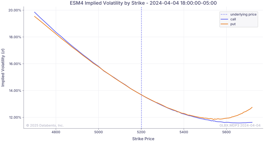
In this example we will use the Historical client to process instrument definition and MBP-1 data to graph implied volatility by strike price for the front-month E-mini S&P 500 Futures (ES) contract. To do this we will request top-of-book data for the front-month ES futures contract using our continuous contract symbology and the entire ES options chain using our parent symbology. We will then filter the options by their underlying, to only consider options for the front-month contract. Finally, we will extract prices for these instruments and use the Black-76 model to graph implied volatility by strike price for the nearest quarterly E-mini S&P 500 (ES) options expiration.

Implied volatility

Implied Volatility (IV) is a key concept in the field of options trading and financial markets. It represents the market's forecast of a likely movement in a security's price. Rather than reflecting historical price changes, implied volatility looks forward into the market's expectations and is often used as an indicator of market sentiment for options trading. Naturally, a higher implied volatility indicates larger price movements are expected.

Black-76 model

The most famous model for calculating implied volatility is the Black-Scholes model. This model is primarily used for pricing equities options. In this example, we will be calculating the implied volatility using options on futures, so we will use an alternative model called the Black-76 model. This model is more appropriate for options on futures, bonds, and other interest rate products.

Typically, the implied volatility is assumed and is used to calculate the price of an option. In this exercise we will invert this operation, and use historical prices to solve for implied volatility, usually denoted as σ (sigma). We cannot solve for this analytically, so we will use the scipy module to find sigma numerically using scipy.optimize.root_scalar.

Dependencies

This example will use the scipy module to perform the implied volatility calculation. The matplotlib package will be used for charting.

These dependencies can be installed with the following:

$ pip install scipy matplotlib

Example

from collections.abc import Iterable
import databento as db
import matplotlib.pyplot as plt
import numpy as np
import pandas as pd
from matplotlib.ticker import PercentFormatter
from scipy.optimize import root_scalar
from scipy.stats import norm

dataset = "GLBX.MDP3"


def black_76(
    S: float,
    K: float,
    T: float,
    sigma: float,
    r: float = 0.05,
    is_call_option: bool = True,
) -> float:
    """
    Calculate an option price from the Black-76 model.

    Parameters
    ----------
    S : float
        Current underlying price.
    K : float
        Option strike price.
    T : float
        Time to expiration in years.
    sigma : float
        Implied volatility, annualized.
    r : float, default 0.05
        The risk free interest rate, annualized.
    is_call_option : bool, default True
        Flag to indicate the option is a call or put.

    Returns
    -------
    float

    """
    d1 = (np.log(S / K) + (sigma**2 / 2) * T) / (sigma * np.sqrt(T))
    d2 = d1 - sigma * np.sqrt(T)
    discount_factor = np.exp(-r * T)

    cp = 1 if is_call_option else -1
    return discount_factor * cp * (S * norm.cdf(cp * d1) - K * norm.cdf(cp * d2))


def get_front_month_symbol(
    parent: str,
    start: pd.Timestamp,
) -> str:
    """
    Get the symbol of the front month futures contract of a given parent symbol.

    Parameters
    ----------
    parent : str
        The parent symbol, such as ES.
    start : pd.Timestamp
        The date to obtain the front month symbol for.

    Returns
    -------
    str

    """
    front_def = client.timeseries.get_range(
        dataset=db.Dataset.GLBX_MDP3,
        schema=db.Schema.DEFINITION,
        symbols=[f"{parent}.c.0"],
        stype_in=db.SType.CONTINUOUS,
        start=start.date(),
        end=(start + pd.Timedelta(days=1)).date(),
    ).to_df()
    return front_def.iloc[0]["raw_symbol"]


def get_options_chain(
    parent: str,
    underlying: str,
    start: pd.Timestamp,
) -> pd.DataFrame:
    """
    Retrieve the definitions of all options contract of the given parent symbol with for the underlying.

    Parameters
    ----------
    parent : str
        The parent symbol, such as ES.
    underlying : str
        The underlying contract for the option.
    start : pd.Timestamp
        The date to obtain the definitions for.

    Returns
    -------
    pd.DataFrame

    """
    options_def = client.timeseries.get_range(
        dataset=dataset,
        schema="definition",
        symbols=f"{parent}.OPT",
        stype_in="parent",
        start=start.date(),
    )

    df = options_def.to_df()
    df = df[df["underlying"] == underlying]
    df = df[df["instrument_class"].isin(("C", "P"))]
    df["years_to_expiration"] = (df["expiration"] - start).dt.days / 365
    return df.sort_values("strike_price")


def get_midprice(
    symbols: Iterable[str],
    start: pd.Timestamp,
    end: pd.Timestamp,
) -> pd.Series:
    """
    Get the last top-of-book midprice for one or more symbols between the `start` and `end` times.

    Parameters
    ----------
    symbols : Iterable[str]
        A collection of symbols to retrieve the midprices for.
    start : pd.Timestamp
        The start time.
    end : pd.Timestamp
        The end time (exclusive).

    Returns
    -------
    pd.Series

    """
    price_df = client.timeseries.get_range(
        dataset=dataset,
        schema="mbp-1",
        symbols=symbols,
        start=start,
        end=end,
    ).to_df()

    price_df = price_df.groupby("symbol").last()
    price_df["midprice"] = np.mean(price_df[["bid_px_00", "ask_px_00"]], axis=1)

    return price_df["midprice"]


def find_sigma(
    row: pd.Series,
) -> float:
    """
    Find the roots of the Black-76 model by varying sigma, implied volatility.

    This function is for use with `pandas.Dataframe.apply`. Each row should contain
    a column for "strike_price", "years_to_expiration", "instrument_class", "midprice",
    and "underlying_price",

    If the optimization fails, `numpy.nan` is returned.

    Parameters
    ----------
    row : pd.Series
        A series of data to process.

    Returns
    -------
    float | numpy.nan

    """

    def f(sigma: float) -> float:
        return row["midprice"] - black_76(
            S=row["underlying_price"],
            K=row["strike_price"],
            T=row["years_to_expiration"],
            sigma=sigma,
            is_call_option=row["instrument_class"] == "C",
        )

    result = root_scalar(f, x0=0.1, x1=0.5)
    if result.converged:
        return result.root
    print(
        f"Could not find sigma for {row['raw_symbol']} with midprice {row['midprice']}",
    )
    return np.nan


# First, create a historical client
client = db.Historical(key="$YOUR_API_KEY")

# Now, define some parameters for the calculation
parent_symbol = "ES"
start = pd.Timestamp("2024-04-04T17:00:00", tz="US/Central")
end = pd.Timestamp("2024-04-04T18:00:00", tz="US/Central")

# Get the front month futures contract for the parent symbol
front_month_symbol = get_front_month_symbol(
    parent=parent_symbol,
    start=start,
)

# Get the definitions for all options with the front-month future as the underlying
options_chain = get_options_chain(
    parent=parent_symbol,
    underlying=front_month_symbol,
    start=start,
)

# Retrieve the midprices for the options and front-month future
midprices = get_midprice(
    symbols=[front_month_symbol, *options_chain["raw_symbol"]],
    start=start,
    end=end,
)

# Then, join the options definitions with the midprices
underlying_price = midprices.loc[front_month_symbol]
options_chain = options_chain.join(midprices, on="symbol").dropna(subset="midprice")
options_chain["underlying_price"] = underlying_price

# Remove options with strike prices far from the underlying price
options_chain = options_chain[
    abs(options_chain["strike_price"] - underlying_price) <= underlying_price * 0.1
]

# Next, find the implied volatility for each option
options_chain["sigma"] = options_chain.apply(
    find_sigma,
    axis=1,
)

# Separate options into calls and puts
call_options = options_chain[options_chain["instrument_class"] == "C"]
put_options = options_chain[options_chain["instrument_class"] == "P"]

# Finally, plot each curve of implied volatility by strike price
plt.axvline(
    underlying_price,
    label="underlying price",
    linestyle=":",
)
plt.plot(
    "strike_price",
    "sigma",
    data=call_options,
    label="call",
)
plt.plot(
    "strike_price",
    "sigma",
    data=put_options,
    label="put",
)
plt.title(f"{front_month_symbol} Implied Volatility by Strike - {end}")
plt.ylabel("Implied Volatility ($\\sigma$)")
plt.xlabel("Strike Price")
plt.gca().yaxis.set_major_formatter(PercentFormatter(1))
plt.legend()
plt.show()