Join options with underlying prices
Info
This example builds off the Join schemas on instrument ID example.
Overview
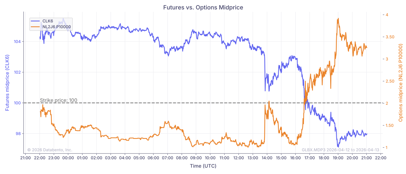
In this example, we'll use the Historical client to get data for futures and options. First, we'll request trades schema data for all options on the volume-based continuous contract and join them with the most recent quote from the MBP-1 schema for the underlying future. We'll also request BBO-1m schema data for the underlying future and a single option and plot the midprice for a full session.
Example
1
2
3
4
5
6
7
8
9
10
11
12
13
14
15
16
17
18
19
20
21
22
23
24
25
26
27
28
29
30
31
32
33
34
35
36
37
38
39
40
41
42
43
44
45
46
47
48
49
50
51
52
53
54
55
56
57
58
59
60
61
62
63
64
65
66
67
68
69
70
71
72
73
74
75
76
77
78
79
80
81
82
83
84
85
86
87
88
89
90
91
92
93
94
95
96
97
98
99
100
101
102
103
104
105
106
107
108
109
110
111
112
113
114
115
116
117
118
119
120
121
122
123
124
125
126
127
128
129
130
131
132
133
134
135
136
137
138
139
140
141
142
143
144
145
146
147
148
149
150
151
152
153
154
155
156
157
158
159
160
161
162
163
164
165
166
167
168
169
170
171
172
173
174
175
176
177
178
179
180
181
182
183
184
185
186
187
188
189
190
191
192
193
194
195
196
197
198
199
200
201
202
203
204
205
206
207
208
import databento as db
import matplotlib.dates as mdates
import matplotlib.pyplot as plt
import pandas as pd

def get_bbo_data(
    dataset: str,
    instrument_id: int,
    start: str,
    end: str,
) -> pd.DataFrame:
    mbp_df = client.timeseries.get_range(
        dataset=dataset,
        schema="bbo-1m",
        symbols=instrument_id,
        stype_in="instrument_id",
        start=start,
        end=end,
    ).to_df(map_symbols=False)
    return mbp_df[["instrument_id", "bid_px_00", "ask_px_00"]]


def plot_option_with_underlying(
    opt_df: pd.DataFrame,
    fut_df: pd.DataFrame,
) -> None:
    opt_df["mid_price"] = (opt_df["bid_px_00"] + opt_df["ask_px_00"]) / 2
    fut_df["mid_price"] = (fut_df["bid_px_00"] + fut_df["ask_px_00"]) / 2

    full_index = pd.date_range(
        start=start,
        end=end,
        freq="1min",
        tz="UTC",
        inclusive="right",
    )
    opt_df = opt_df.reindex(full_index).ffill().astype(opt_df.dtypes)
    fut_df = fut_df.reindex(full_index).ffill().astype(fut_df.dtypes)

    opt_symbol = opt_df["raw_symbol"].iloc[0]
    fut_symbol = opt_df["underlying"].iloc[0]

    fig, ax1 = plt.subplots(figsize=(14, 6))

    ax1.plot(fut_df.index, fut_df["mid_price"], color="C0", label=fut_symbol)
    ax1.set_ylabel(f"Futures midprice ({fut_symbol})", color="C0")
    ax1.tick_params(axis="y", labelcolor="C0")

    strike = opt_df["strike_price"].iloc[0]
    ax1.axhline(y=strike, color="gray", linestyle="--")
    ax1.text(
        x=fut_df.index[0],
        y=strike,
        s=f"Strike price: {strike:.0f}",
        color="gray",
        va="bottom",
        ha="left",
    )

    ax2 = ax1.twinx()
    ax2.plot(opt_df.index, opt_df["mid_price"], color="C1", label=opt_symbol)
    ax2.set_ylabel(f"Options midprice ({opt_symbol})", color="C1")
    ax2.tick_params(axis="y", labelcolor="C1")

    ax1.xaxis.set_major_formatter(mdates.DateFormatter("%H:%M"))
    ax1.xaxis.set_major_locator(mdates.HourLocator(interval=1))

    ax1.set_title("Futures vs. Options Midprice")
    ax1.set_xlabel("Time (UTC)")

    lines1, labels1 = ax1.get_legend_handles_labels()
    lines2, labels2 = ax2.get_legend_handles_labels()
    ax1.legend(lines1 + lines2, labels1 + labels2, loc="upper left")

    ax1.grid(True)
    ax2.grid(False)

    fig.tight_layout()
    plt.show()


# Create a historical client
client = db.Historical("$YOUR_API_KEY")

# Set parameters
dataset = "GLBX.MDP3"
symbol = "CL.v.0"
start = "2026-04-12T22:00:00"
end = "2026-04-13T21:00:00"

# Get symbol mapping for the continuous contract
symbol_map = client.symbology.resolve(
    dataset=dataset,
    symbols=symbol,
    stype_in="continuous",
    stype_out="instrument_id",
    start_date="2026-04-12",
)
# Get instrument ID for the resolved futures contract
fut_id = int(symbol_map["result"][symbol][0]["s"])

# Get all option definitions
def_df = client.timeseries.get_range(
    dataset=dataset,
    symbols="ALL_SYMBOLS",
    schema="definition",
    start="2026-04-12",
).to_df()

# Filter for options with the continuous contract as an underlying
opt_def_df = def_df[
    (def_df["user_defined_instrument"] == db.UserDefinedInstrument.NO)
    & (def_df["instrument_class"].isin((db.InstrumentClass.CALL, db.InstrumentClass.PUT)))
    & (def_df["underlying_id"] == fut_id)
]
opt_def_df = opt_def_df[
    [
        "ts_event",
        "expiration",
        "raw_symbol",
        "instrument_id",
        "asset",
        "strike_price",
        "underlying",
        "underlying_id",
        "instrument_class",
    ]
]

# Get trades data for the filtered options
opt_trades_df = (
    client.timeseries.get_range(
        dataset=dataset,
        schema="trades",
        symbols=[f"{x}.OPT" for x in opt_def_df["asset"].unique()],
        stype_in="parent",
        start=start,
        end=end,
    )
    .to_df()
    .rename(columns={"size": "trade_size", "price": "trade_price", "side": "trade_side"})
)

# Join options with their definitions
opt_df = (
    opt_trades_df.reset_index()
    .merge(
        opt_def_df.reset_index(),
        on="instrument_id",
        how="inner",
        suffixes=("", "_def"),
    )
    .set_index("ts_recv")
    .sort_index()
)

fut_mbp_df = client.timeseries.get_range(
    dataset=dataset,
    schema="mbp-1",
    symbols=fut_id,
    stype_in="instrument_id",
    start=start,
    end=end,
).to_df()
fut_mbp_df = fut_mbp_df.rename(
    columns={
        "bid_px_00": "underlying_bid",
        "ask_px_00": "underlying_ask",
    },
)[["underlying_bid", "underlying_ask"]]

# Join most recent underlying bid/ask with options trades
df = pd.merge_asof(
    opt_df,
    fut_mbp_df,
    left_index=True,
    right_index=True,
    direction="backward",
)

print(
    df[
        [
            "ts_event",
            "instrument_id",
            "raw_symbol",
            "trade_price",
            "trade_size",
            "trade_side",
            "strike_price",
            "instrument_class",
            "expiration",
            "underlying_bid",
            "underlying_ask",
        ]
    ],
)

# 42963414 is the `instrument_id` for NL2J6 P10000
opt_id = 42963414
opt_bbo_df = get_bbo_data(dataset, opt_id, start, end)
opt_bbo_df = (
    opt_bbo_df.reset_index().merge(opt_def_df, on="instrument_id", how="left").set_index("ts_recv")
)

fut_bbo_df = get_bbo_data(dataset, fut_id, start, end)

plot_option_with_underlying(opt_bbo_df, fut_bbo_df)
Result
We can see all trades for options that have the volume-based continuous contract as an underlying.
1
2
3
4
5
6
7
8
9
10
11
12
13
14
15
                                                               ts_event  instrument_id    raw_symbol  trade_price  trade_size  ... strike_price  instrument_class                expiration underlying_bid  underlying_ask
ts_recv                                                                                                                        ...
2026-04-12 22:00:00.356333832+00:00           2026-04-12 22:00:00+00:00       42157669    LOK6 C9900         6.01           1  ...        99.00                 C 2026-04-16 18:30:00+00:00            NaN             NaN
2026-04-12 22:00:00.356370138+00:00           2026-04-12 22:00:00+00:00       42180553    LOK6 P8200         0.39           1  ...        82.00                 P 2026-04-16 18:30:00+00:00            NaN             NaN
2026-04-12 22:00:00.357402871+00:00           2026-04-12 22:00:00+00:00       42511805  ML2J6 C10000         2.40           2  ...       100.00                 C 2026-04-13 18:30:00+00:00            NaN             NaN
2026-04-12 22:00:00.357526014+00:00           2026-04-12 22:00:00+00:00       42639465   ML2J6 P9100         0.74           1  ...        91.00                 P 2026-04-13 18:30:00+00:00            NaN             NaN
2026-04-12 22:00:00.357609934+00:00           2026-04-12 22:00:00+00:00       42963412   NL2J6 P9600         0.99           1  ...        96.00                 P 2026-04-14 18:30:00+00:00            NaN             NaN
...                                                                 ...            ...           ...          ...         ...  ...          ...               ...                       ...            ...             ...
2026-04-13 20:57:18.223377118+00:00 2026-04-13 20:57:18.222967937+00:00       42308894    LOK6 P8500         0.27           1  ...        85.00                 P 2026-04-16 18:30:00+00:00          97.96           97.98
2026-04-13 20:57:18.223891862+00:00 2026-04-13 20:57:18.223423419+00:00       42308894    LOK6 P8500         0.27           1  ...        85.00                 P 2026-04-16 18:30:00+00:00          97.96           97.98
2026-04-13 20:57:19.267462126+00:00 2026-04-13 20:57:19.267057293+00:00       42631933   WL3J6 C9775         3.03           1  ...        97.75                 C 2026-04-15 18:30:00+00:00          97.97           97.99
2026-04-13 20:58:04.991697756+00:00 2026-04-13 20:58:04.983728493+00:00       42958534  NL2J6 C10100         0.91           1  ...       101.00                 C 2026-04-14 18:30:00+00:00          97.94           97.96
2026-04-13 20:58:38.292464827+00:00 2026-04-13 20:58:38.292053561+00:00         379004    LOK6 P7000         0.02           1  ...        70.00                 P 2026-04-16 18:30:00+00:00          97.97           97.99

[17262 rows x 11 columns]
Now we'll plot the midprice of the underlying future and a single option for the duration of a full session. In this example, the option NL2J6 P10000 expires on 2026-04-14.