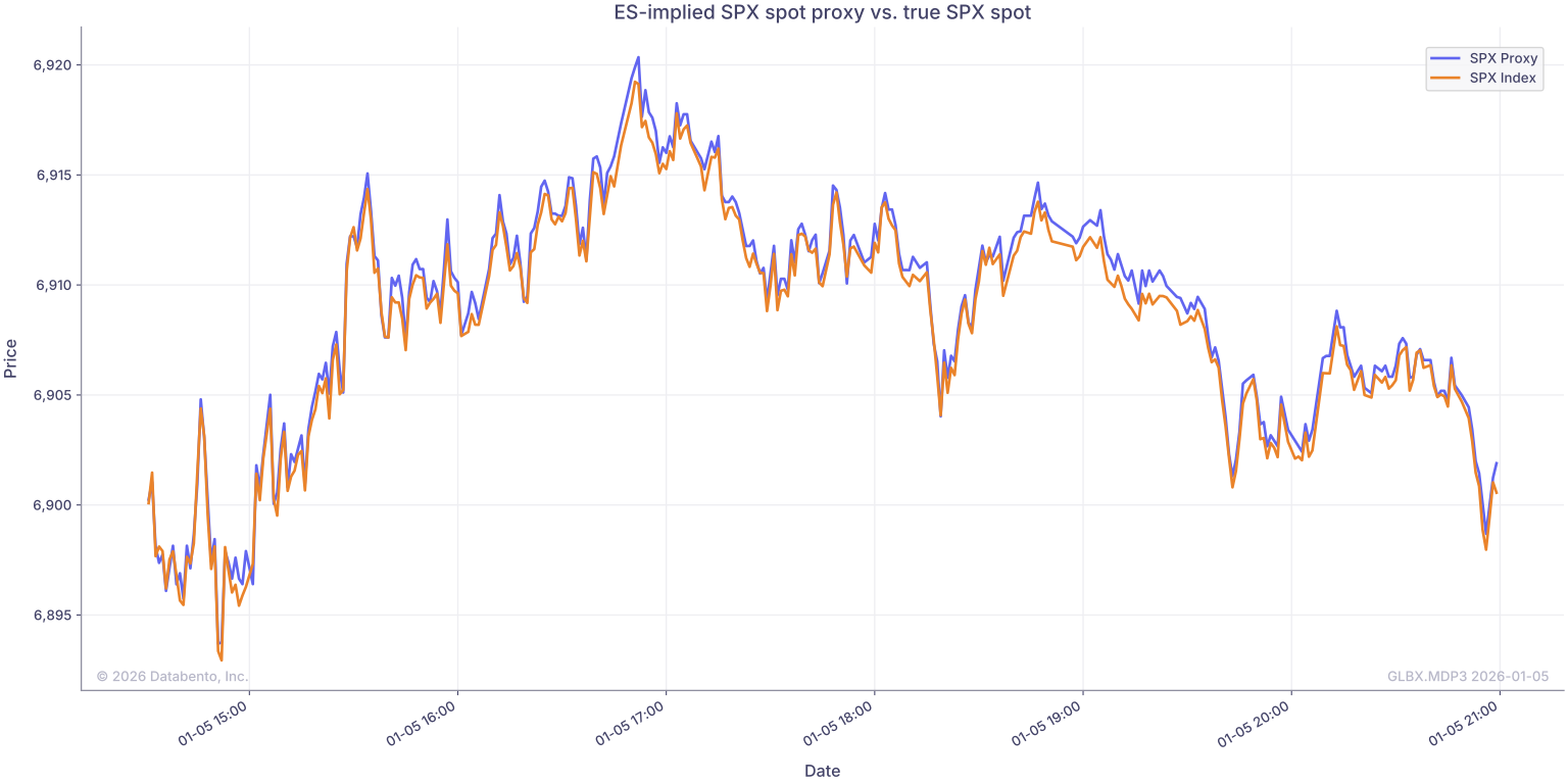
In this example, we'll explore how to estimate the implied spot price for the S&P 500 Index using best bid and offer (BBO) data from the ES curve with Databento's Historical client. We will then validate the implied price against the true underlying index value from our Databento Core Indices dataset.

Because ES futures trade nearly continuously and update more frequently than the published SPX cash index, they can be used to construct a real-time proxy for the underlying index level.

Futures overview and cost of carry

A futures contract is a standardized legal agreement to buy or sell an underlying asset at a specified price on a future date. Some futures, including ES futures, are cash-settled rather than settled through delivery of the underlying asset.

The price of a futures contract at a given expiration is determined by the current spot price, adjusted for factors associated with carrying exposure to the underlying asset until expiration. This adjustment is commonly referred to as the "net cost of carry."

For equity index futures, the net cost of carry primarily reflects the financing cost of purchasing the underlying portfolio and the dividend income forgone by holding the futures contract instead.

Under the standard model, the futures price can be expressed using the risk-free interest rate and the continuous dividend yield as follows:

F_{i} = S \cdot e^{(R - D) T_{i}}

Where:

$F_{i}$ is the i-th futures contract price
$S$ is the current spot price of the underlying asset
$R$ is the risk-free interest rate
$D$ is the continuous dividend yield
$T_{i}$ is the time to expiration of the i-th futures contract

Solving for the spot price

Interest rates and expected dividends may be difficult to source. However, because ES futures trade across multiple expirations, we can use a mathematical trick to infer their combined effect from the futures curve. If we assume that the continuously compounded net carry rate is approximately constant across the first two maturities, we can estimate an implied net carry rate from their observed prices and use it to recover the underlying spot price.

Info
It is important to note that this assumption simplifies the true nature of the net cost of carry. In practice, dividends are paid on discrete dates and may be concentrated unevenly across quarters. Similarly, interest rates also vary by term and are often modeled as piece-wise functions with knots on FOMC days.
We are also assuming that the implied net carry rate remains constant across maturities.

For the first and second contracts:

F_{1} = S \cdot e^{(R - D) T_{1}}

F_{2} = S \cdot e^{(R - D) T_{2}}

Dividing the second equation by the first eliminates the unknown spot price:

\frac{F _{2}}{F _{1}} = e^{(R - D) (T_{2} - T_{1})}

Taking the natural logarithm of both sides yields:

ln (\frac{F _{2}}{F _{1}}) = (R - D) (T_{2} - T_{1})

We can therefore estimate the net carry rate as:

R - D = \frac{ln ( \frac{F _{2}}{F _{1}} )}{T _{2} - T _{1}}

Now that we have found an estimate for the net carry rate, we can substitute it into the original futures-pricing equation and solve for spot:

S = \frac{F _{1}}{e ^{(R - D) T_{1}}}

Substituting the estimated value of $R - D$ , we obtain an ES-implied proxy for the SPX spot price:

S = \frac{F _{1}}{exp \frac{ln ( \frac{F _{2}}{F _{1}} )}{T _{2} - T _{1}} \cdot T _{1}}

With this equation, implementing the calculation using the API becomes straightforward:

Python

      
    
import databento as db
import matplotlib.pyplot as plt
import numpy as np
import pandas as pd

# Create a historical client
client = db.Historical(key="YOUR_API_KEY")

# Set time range
start = "2026-01-05T00:00:00"
end = "2026-01-05T21:00:00"

# Set dataset and symbols
dataset = "GLBX.MDP3"
symbols = ["ES.v.0", "ES.v.1"]

# Get 1-second BBO for the front two continuous ES contracts (ES.v.0, ES.v.1)
es = client.timeseries.get_range(
    dataset=dataset,
    symbols=symbols,
    start=start,
    end=end,
    schema="bbo-1s",
    stype_in="continuous",
    stype_out="instrument_id",
)
es_df = es.to_df()

# Get definitions to map each instrument to its expiration date
definitions = client.timeseries.get_range(
    dataset=dataset,
    symbols=symbols,
    start=start,
    end=end,
    schema="definition",
    stype_in="continuous",
)
definitions_df = definitions.to_df()

# Build a map from instrument_id to expiration
expiration_map = definitions_df.groupby("instrument_id")["expiration"].first().to_dict()

# Attach each row's expiration to the BBO DataFrame
es_df["expiration"] = es_df["instrument_id"].map(expiration_map)

# Time to expiration in years (T_i), and the mid price as our price proxy
es_df["time_to_expire"] = (es_df["expiration"] - es_df["ts_event"]).dt.total_seconds() / (365 * 24 * 60 * 60)
es_df["mid"] = (es_df["bid_px_00"] + es_df["ask_px_00"]) / 2

# Split into the first (F_1) and second (F_2) contracts
es0 = es_df[es_df["symbol"] == "ES.v.0"][["mid", "time_to_expire"]]
es1 = es_df[es_df["symbol"] == "ES.v.1"][["mid", "time_to_expire"]]

# Estimate the net carry rate (R - D) = ln(F_2/F_1) / (T_2 - T_1)
r_d = (np.log(es1["mid"] / es0["mid"])) / (es1["time_to_expire"] - es0["time_to_expire"])

# Back out the implied spot: S = F_1 / e^[(R - D) * T_1]
spx = es0["mid"] / np.exp(r_d * es0["time_to_expire"])

# Combine the prices into a combined DataFrame
proxy_df = pd.DataFrame({"es0": es0["mid"], "es1": es1["mid"], "spx": spx})
print(proxy_df.head(5))

Python

      
    
                                es0       es1          spx
ts_recv
2026-01-05 00:00:00+00:00  6907.125  6958.375  6864.956430
2026-01-05 00:00:01+00:00  6907.375  6958.375  6865.410758
2026-01-05 00:00:02+00:00  6907.375  6958.625  6865.206449
2026-01-05 00:00:03+00:00  6907.500  6958.625  6865.433613
2026-01-05 00:00:04+00:00  6907.250  6958.375  6865.183636

In just a few lines of code, we have created an SPX index proxy that updates more quickly than the true index value. However, we still need to validate its accuracy.

Validation

We can use Databento's Core Indices dataset to request the actual underlying index value, check the accuracy of our estimate, and plot the two time series against one another:

Python

      
    
# Create a request using the DBIX.CORE dataset.
index = client.timeseries.get_range(
    dataset="DBIX.CORE",
    symbols="SPX",
    start=start,
    end=end,
    schema="bbo-1m",
)
index_df = index.to_df()
index_df["idx"] = (index_df["bid_px_00"] + index_df["ask_px_00"]) / 2

# Combine data, keeping only rows from the DBIX DataFrame
prices_df = pd.merge(left=index_df[["idx"]],
                    right=proxy_df,
                    how="left",
                    left_index=True,
                    right_index=True)
prices_df = prices_df[prices_df["spx"].notnull()]

# Plot the implied SPX proxy against the true index price
plt.figure(figsize=(16, 8))
prices_df["spx"].plot(label="SPX Proxy")
prices_df["idx"].plot(label="SPX Index")
plt.title("ES-implied SPX spot proxy vs. true SPX spot")
plt.xlabel("Date")
plt.ylabel("Price")
plt.legend()
plt.show()

SPX implied proxy

Error

To measure the error between our SPX index proxy and the true SPX index, we can use the Root Mean Squared Error (RMSE), which quantifies the differences (residuals) between predicted and actual values. It squares each difference to penalize larger errors and eliminate negative errors, averages the squared differences, and takes the square root to return the error to the original units. The exact equation is:

RMSE = \frac{1}{n} i = 1 \sum n (\hat{S}_{i} - S_{i})^{2}

Where:

$\hat{S}_{i}$ is the ES-implied proxy at observation i
$S_{i}$ is the true index value at observation i
$n$ is the number of observations

We can achieve this quite easily in Python with no additional packages:

Python

# Calculate RMSE
rmse = np.sqrt(((prices_df["spx"] - prices_df["idx"])**2).sum() / len(prices_df))
print("Root Mean Squared Error:", round(rmse, 4))

Root Mean Squared Error: 0.6386

So our estimate is only off by an RMSE of ~0.64 index points. This is an excellent result, but to ensure this metric is reasonable, we still need to inspect the distribution of errors.

Residuals

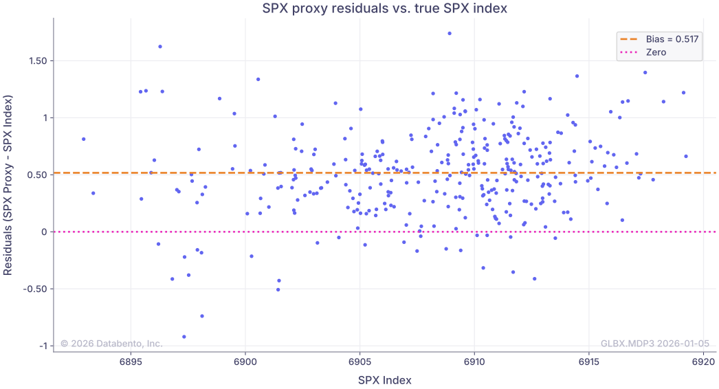
For a better idea of how the errors are distributed, we can create a residual plot. This plot displays each error as a point on a graph, allowing us to visually inspect whether our estimate is systematically biased in one direction. We can find a consistent bias by measuring the average size of our residuals:

Bias = \frac{1}{n} i = 1 \sum n (\hat{S}_{i} - S_{i})

We can calculate this value in Python and plot it alongside our residuals plot:

Python

      
    
# Calculate mean error
bias = (prices_df["spx"] - prices_df["idx"]).mean()

# Plot residuals vs. true index price.
plt.scatter(x=prices_df["idx"],
            y=prices_df["spx"] - prices_df["idx"]
            )
plt.axhline(bias, color="C1", linestyle="--", label=f"Bias = {bias:.3f}")
plt.axhline(0, color="C2", linestyle=":", label="Zero")
plt.xlabel("SPX Index")
plt.ylabel("Residuals (SPX Proxy - SPX Index)")
plt.title("SPX proxy residuals vs. true SPX index")
plt.legend()
plt.show()

print("Bias:", round(bias, 4))

SPX residual plot

Bias: 0.517

This plot shows that our estimate was consistently about half an index point too high, indicating that our simplified cost-of-carry model may introduce structural bias. This bias may vary across days due to the non-linear nature of the cost of carry. However, given that error is measured as follows:

RMSE^{2} = Bias^{2} + σ^{2}

We can calculate the standard deviation of our estimate around the bias.

σ = RMSE^{2} - Bias^{2}

Then, we can calculate this value in Python:

Python

variance = rmse**2 - bias**2
print("Standard Deviation:", round(variance**0.5))

Standard Deviation: 0.375

Our estimate has a standard deviation of less than 1/2 of an index point around our bias, meaning that our proxy is quite robust. We can use this proxy to find at-the-money options strikes, find a continuous index level outside of regular trading hours, and compute realized volatility on a tick-by-tick basis.