Filter options by moneyness
Overview
In this example, we'll calculate the moneyness of SPXW options and filter to strikes within 5% of the ATM price. We'll calculate moneyness for each option by combining SPXW option definitions and statistics from Databento's OPRA dataset with SPX index values from the Databento Core Indices dataset.
Moneyness
Moneyness describes where an option's strike sits relative to the current price of the underlying.
The moneyness of an option is separated into three trading states:
- In-the-money (ITM): The option has positive intrinsic value.
- At-the-money (ATM): The option's strike price is almost identical to the market price of the underlying asset.
- Out-of-the-money (OTM): The option has no intrinsic value.
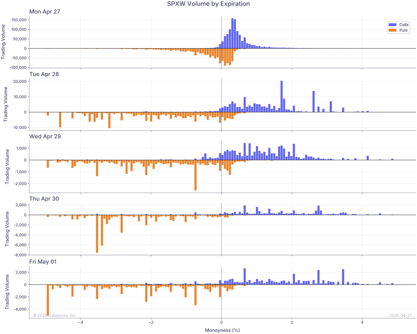
Options closer to ATM typically have higher trading volume.
For any option:
Moneyness=SK−1Where:
- K is the strike price of the contract
- S is the current price of the underlying asset
A negative value places the strike below spot, which is in-the-money for a call and out-of-the-money for a put. The opposite is true for a positive value. Both the sign and the contract type determine the state of an option.
For easier readability, we will multiply this value by 100 to express moneyness as a percentage rather than a decimal.
Calculating moneyness
To calculate moneyness, we'll use the definition schema to retrieve the necessary information for each option, such as expiration, strike_price, and instrument_class. We'll then pull the spot price at market open using the OHLCV schema.

import databento as db
import pandas as pd

# Create a historical client
client = db.Historical(key="$YOUR_API_KEY")

# Fetch data for all expirations for the week of Monday, April 27
start = "2026-04-27"

# Fetch the SPX index price from market open
spx_df = client.timeseries.get_range(
    dataset="DBIX.CORE",
    schema="ohlcv-1m",
    symbols=["SPX"],
    start=start + "T13:30",
    end=start + "T13:31",
).to_df()
spx = spx_df[spx_df["symbol"] == "SPX"]["open"].iloc[0]

# Fetch SPXW options definitions
spxw_definitions = client.timeseries.get_range(
    dataset="OPRA.PILLAR",
    schema="definition",
    symbols=["SPXW.OPT"],
    stype_in="parent",
    start=start,
).to_df()

# Filter to outright contracts expiring by the end of the week
friday_expiry = pd.to_datetime(start, utc=True) + pd.Timedelta(days=4)
spxw_definitions = spxw_definitions[spxw_definitions["expiration"] <= friday_expiry]
spxw_definitions = spxw_definitions[spxw_definitions["instrument_class"].isin(["P", "C"])]

# Drop all unnecessary rows for this process
spxw_metadata = spxw_definitions[["instrument_id", "strike_price", "expiration", "instrument_class"]]

# Calculate Moneyness per contract (For the sake of this example, we convert to a percentage by multiplying by 100)
spxw_metadata["moneyness"] = (spxw_metadata["strike_price"] / spx - 1) * 100

print(spxw_metadata.head())
                                     instrument_id  strike_price                expiration instrument_class  moneyness
ts_recv
2026-04-27 10:30:04.059606168+00:00     1191185088        6500.0 2026-05-01 00:00:00+00:00                C  -9.125480
2026-04-27 10:30:04.069618621+00:00     1191185095        7150.0 2026-05-01 00:00:00+00:00                C  -0.038027
2026-04-27 10:30:04.069618621+00:00     1191185096        5200.0 2026-05-01 00:00:00+00:00                C -27.300384
2026-04-27 10:30:04.079627286+00:00     1191185103        5950.0 2026-05-01 00:00:00+00:00                P -16.814862
2026-04-27 10:30:04.079627286+00:00     1191185104        6300.0 2026-05-01 00:00:00+00:00                C -11.921619
Visualizing activity by strike
Now that we have calculated the moneyness of each strike price, we can visualize the trading activity within 5% of the opening ATM price. A single SPXW expiration lists strikes across a range far wider than the underlying is likely to move, and most of them barely trade, so any workflow that consumes the chain could benefit from cutting it down to an active region.
import databento as db
import matplotlib.pyplot as plt
import numpy as np
import pandas as pd

# Create a historical client
client = db.Historical(key="$YOUR_API_KEY")

# Fetch data for all expirations for the week of Monday, April 27
start = "2026-04-27"

# Fetch the SPX index price from market open
spx_df = client.timeseries.get_range(
    dataset="DBIX.CORE",
    schema="ohlcv-1m",
    symbols=["SPX"],
    start=start + "T13:30",
    end=start + "T13:31",
).to_df()
spx = spx_df[spx_df["symbol"] == "SPX"]["open"].iloc[0]

# Fetch SPXW options definitions
spxw_definitions = client.timeseries.get_range(
    dataset="OPRA.PILLAR",
    schema="definition",
    symbols=["SPXW.OPT"],
    stype_in="parent",
    start=start,
).to_df()

# Filter to outright contracts expiring by the end of the week
friday_expiry = pd.to_datetime(start, utc=True) + pd.Timedelta(days=4)
spxw_definitions = spxw_definitions[spxw_definitions["expiration"] <= friday_expiry]
spxw_definitions = spxw_definitions[spxw_definitions["instrument_class"].isin(["P", "C"])]

# Drop all unnecessary rows for this process
spxw_metadata = spxw_definitions[["instrument_id", "strike_price", "expiration", "instrument_class"]]

# Calculate Moneyness per contract (For the sake of this example, we convert to a percentage by multiplying by 100)
spxw_metadata["moneyness"] = (spxw_metadata["strike_price"] / spx - 1) * 100

# Fetch SPXW options statistics
spxw_statistics = client.timeseries.get_range(
    dataset="OPRA.PILLAR",
    schema="statistics",
    symbols=["SPXW.OPT"],
    stype_in="parent",
    start=start,
).to_df()

# Include only daily volume statistics
spxw_volumes = spxw_statistics[spxw_statistics["stat_type"] == db.StatType.CLEARED_VOLUME][["instrument_id", "quantity"]]
spxw_volumes = spxw_volumes.groupby("instrument_id").last().reset_index().rename(columns={"quantity": "volume"})

# Merge the metadata and volume dataframes
spxw = pd.merge(spxw_volumes, spxw_metadata, on="instrument_id")

# Create a reusable function to plot the volume data for each expiration date
def volume_plots(axes, plot_df, expiries, alpha=1):
    for ax, expiry in zip(axes, expiries):
        # Filter the dataframe to only include options for the current expiration date
        expiry_df = plot_df[plot_df["expiration"] == expiry]
        puts = expiry_df[expiry_df["instrument_class"] == "P"]
        calls = expiry_df[expiry_df["instrument_class"] == "C"]

        x_values = np.sort(expiry_df["moneyness"].unique())
        bar_width = np.median(np.diff(x_values)) * 0.85 # Bar width will be 85% of the median price difference between strikes

        # Plot the volume for calls and puts as bars, with calls above the x-axis and puts below the x-axis
        ax.bar(calls["moneyness"], calls["volume"], width=bar_width, label="Calls", alpha=alpha, color="C0")
        ax.bar(puts["moneyness"], -puts["volume"], width=bar_width, label="Puts", alpha=alpha, color="C1")

        # Add a vertical line at moneyness = 0 and a horizontal line at volume = 0
        ax.axvline(0, linestyle="--", linewidth=1)
        ax.axhline(0, linewidth=0.8, color="black")
        ax.set_title(pd.Timestamp(expiry).strftime("%a %b %d"), loc="left")
        ax.set_ylabel("Trading Volume")

# Filter to only include options that are within 5% of the SPX index price
plot_df = spxw[spxw["moneyness"].between(-5, 5)]

# Create a list of unique expiration dates for the options
expiries = sorted(plot_df["expiration"].unique())

# Create the subplots for each expiration date
fig, axes = plt.subplots(nrows=len(expiries), ncols=1, figsize=(15, 12), sharex=True)

volume_plots(axes, plot_df, expiries)

axes[-1].set_xlabel("Moneyness (%)")
axes[0].legend()
fig.suptitle("SPXW Volume by Expiration", fontsize=16)
plt.show()