In this example, we will use the VIX to define a volatility-adjusted active strike range across SPXW expirations from the OPRA feed using SPX and VIX index values from Databento's Databento Core Indices dataset.

Info
This article is a continuation of our Filter options by moneyness example. For more details on moneyness, visit that page first.

The VIX

The VIX, or Cboe Volatility Index, is a market index that measures the S&P 500's anticipated volatility in the near future. VIX is derived from the SPX option chain and expresses expected 30-day volatility in annualized terms. For this example, we will focus on 0DTE-5DTE options contracts, so we will instead use shorter-term versions of the VIX: VIX1D and VIX9D, which measure the S&P 500's expected volatility for the current trading day and the next 9 days respectively. Then, we will use these two points to interpolate the implied total variance for each expiration. We use variance instead of volatility here because variance is additive over time.

To do this, we first need to convert volatility to annualized variance by squaring:

Va r_{1 D} = (VIX1D)^{2}

Va r_{9 D} = (VIX9D)^{2}

Next, we will account for the time fraction of each index to get the actual total variance expected over their respective horizons:

Total Var_{1 D} = Va r_{1 D} \times \frac{1}{365}

Total Var_{9 D} = Va r_{9 D} \times \frac{9}{365}

We then linearly interpolate for the target day by calculating where it sits proportionally between day 1 and day 9:

Total Var_{N D} = Total Var_{1 D} + (\frac{N - 1}{9 - 1}) \times (Total Var_{9 D} - Total Var_{1 D})

Finally, we take the square root of the total variance to get the expected move over n days. This converts the variance back into a percentage move, the same unit as moneyness:

Expected Move_{N D} = Total Var_{N D}

We can achieve this very simply in Python:

Python

      
    
import databento as db
import matplotlib.pyplot as plt
import numpy as np
import pandas as pd

#  Create a historical client
client = db.Historical(key="YOUR_API_KEY")

# Fetch data for all expirations for the week of Monday, April 27
start = "2026-04-27"

# Get the opening values for the VIX (not available exactly at open, since the VIX is calculated from SPX options)
vix_df = client.timeseries.get_range(
    dataset="DBIX.CORE",
    schema="ohlcv-1s",
    symbols=["VIX1D", "VIX9D"],
    start=start + "T13:31",
    end=start + "T13:32",
).to_df()
vix1d = vix_df[vix_df["symbol"] == "VIX1D"]["open"].iloc[0]
vix9d = vix_df[vix_df["symbol"] == "VIX9D"]["open"].iloc[0]

# Square the indices to get annualized variances
var_1d = vix1d ** 2
var_9d = vix9d ** 2

# Convert to annualized variances for the respective horizons
total_var_1d = var_1d * (1 / 365)
total_var_9d = var_9d * (9 / 365)

# Interpolate days 1 through 5
expected_moves = {}

for n in range(1, 6):
    weight = (n - 1) / (9 - 1)
    total_var_n = (total_var_1d + weight * (total_var_9d - total_var_1d))

    # Convert to expected move and map to expiration
    expected_moves[pd.to_datetime(start, utc=True) + pd.Timedelta(days=n - 1)] = total_var_n ** 0.5

# Now that we have interpolated the expected moves for each expiry,
# we can filter for all strikes within one standard deviation of the spot.
# Under normal assumptions, there is a ~68% chance that the spot price will settle within this band.

# Fetch the SPX index price from market open to calculate moneyness
spx_df = client.timeseries.get_range(
    dataset="DBIX.CORE",
    schema="ohlcv-1m",
    symbols=["SPX"],
    start=start + "T13:30",
    end=start + "T13:31",
).to_df()
spx = spx_df[spx_df["symbol"] == "SPX"]["open"].iloc[0]

# Fetch SPXW options definitions
spxw_definitions = client.timeseries.get_range(
    dataset="OPRA.PILLAR",
    schema="definition",
    symbols=["SPXW.OPT"],
    stype_in="parent",
    start=start,
).to_df()

# Filter to outright contracts expiring by the end of the week
friday_expiry = pd.to_datetime(start, utc=True) + pd.Timedelta(days=4)
spxw_definitions = spxw_definitions[spxw_definitions["expiration"] <= friday_expiry]
spxw_definitions = spxw_definitions[spxw_definitions["instrument_class"].isin(["P", "C"])]

# Drop all unnecessary rows for this process
spxw_metadata = spxw_definitions[["instrument_id", "strike_price", "expiration", "instrument_class"]]

# Calculate Moneyness per contract (For the sake of this example, we convert to a percentage by multiplying by 100)
spxw_metadata["moneyness"] = (spxw_metadata["strike_price"] / spx - 1) * 100

# Fetch SPXW options statistics
spxw_statistics = client.timeseries.get_range(
    dataset="OPRA.PILLAR",
    schema="statistics",
    symbols=["SPXW.OPT"],
    stype_in="parent",
    start=start,
).to_df()

# Include only daily volume statistics
spxw_volumes = spxw_statistics[spxw_statistics["stat_type"] == db.StatType.CLEARED_VOLUME][["instrument_id", "quantity"]]
spxw_volumes = spxw_volumes.groupby("instrument_id").last().reset_index().rename(columns={"quantity": "volume"})

# Merge the metadata and volume dataframes
spxw = pd.merge(spxw_volumes, spxw_metadata, on="instrument_id")

# Create a reusable function to plot the volume data for each expiration date
def volume_plots(axes, plot_df, expiries, alpha=1):
    for ax, expiry in zip(axes, expiries):
        # Filter the dataframe to only include options for the current expiration date
        expiry_df = plot_df[plot_df["expiration"] == expiry]
        puts = expiry_df[expiry_df["instrument_class"] == "P"]
        calls = expiry_df[expiry_df["instrument_class"] == "C"]

        x_values = np.sort(expiry_df["moneyness"].unique())
        bar_width = np.median(np.diff(x_values)) * 0.85 # Bar width will be 85% of the median price difference between strikes

        # Plot the volume for calls and puts as bars, with calls above the x-axis and puts below the x-axis
        ax.bar(calls["moneyness"], calls["volume"], width=bar_width, label="Calls", alpha=alpha, color="C0")
        ax.bar(puts["moneyness"], -puts["volume"], width=bar_width, label="Puts", alpha=alpha, color="C1")

        # Add a vertical line at moneyness = 0 and a horizontal line at volume = 0
        ax.axvline(0, linestyle="--", linewidth=1)
        ax.axhline(0, linewidth=0.8, color="black")
        ax.set_title(pd.Timestamp(expiry).strftime("%a %b %d"), loc="left")
        ax.set_ylabel("Trading Volume")

# Filter to only include options that are within 5% of the SPX index price
plot_df = spxw[spxw["moneyness"].between(-5, 5)]

# Create a list of unique expiration dates for the options
expiries = sorted(plot_df["expiration"].unique())

# Create a mask for options that are within the expected move range and those that are outside of it
inside_range_mask = abs(plot_df["moneyness"]) < plot_df["expiration"].map(expected_moves)
outside_range_mask = abs(plot_df["moneyness"]) > plot_df["expiration"].map(expected_moves)

# Use the function defined above to plot the options that are within the expected move range
# and those that are outside of it, with different alpha values for each
fig, axes = plt.subplots(nrows=len(expiries), ncols=1, figsize=(15, 12), sharex=True)
volume_plots(axes, plot_df[inside_range_mask], expiries, alpha=1)
axes[0].legend() # Avoid duplicate legends by only adding it to the first subplot
volume_plots(axes, plot_df[outside_range_mask], expiries, alpha=0.3)

# Add vertical lines to indicate the expected move range for each expiration date
for i in range(len(expiries)):
    axes[i].axvspan(-expected_moves[expiries[i]], expected_moves[expiries[i]], alpha=0.08)
    axes[i].axvline(-expected_moves[expiries[i]], linestyle=":")
    axes[i].axvline( expected_moves[expiries[i]], linestyle=":")
    axis_title = f"{pd.Timestamp(expiries[i]).strftime('%a %b %d')} — Volatility range: ±{expected_moves[expiries[i]]:.2f}%"
    axes[i].set_title(axis_title, loc="left")

axes[-1].set_xlabel("Moneyness (%)")
fig.suptitle("SPXW Volume by Expiration", fontsize=16)
plt.show()

Strikes filtered by volatility

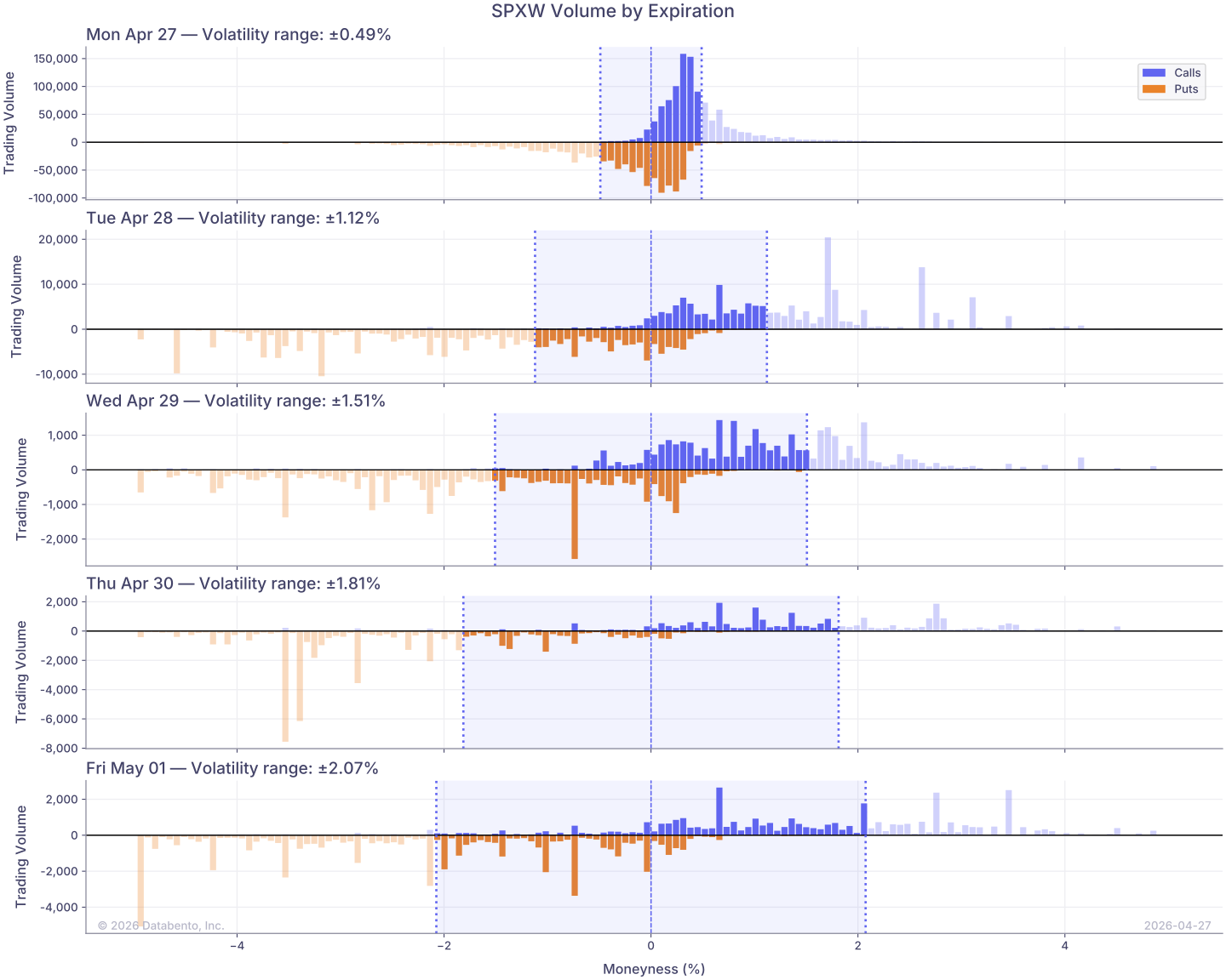
Each shaded band now scales with the expiration's expected volatility rather than by a fixed percentage. Because we have the moneyness mapped to each instrument_id, we can easily subscribe to only the contracts we have identified as liquid for each expiration.